I have figured out how the algorithm works in the paper. I'm posting this answer just in case someone else is looking for the same problem.
First, note that as people have mentioned, this problem is underspecified for $M>2$. There are $2^M$ possible masses for the joint distribution of $M$ Bernoullis and there are $1 + M +\binom{M}{2}$ constraints. (The 1 is from the sum of the probability masses to be 1, $M$ is from $M$ variances, and $\binom{M}{2}$ are from the pairwise correlations.)
However, sampling from such distributions is often necessary, for instance in simulating clinical trials, the default risk of corporate bonds, or slashing risk in L2 blockchains.
The following algorithm works for practical purposes but note that the distribution it finds is not unique and it will fail silently if there is no such distribution. Hence, always verify the sample correlations.
Intuition
Let's start with the $M=2$ case. Suppose we want to sample from the joint distribution of two Bernoulli distributions with parameters $p_1$ and $p_2$ and their (Pearson) correlation $\rho$.
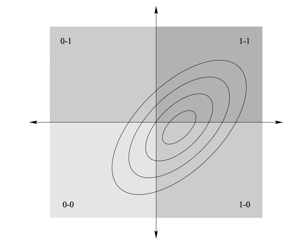
The first insight is observing that we can sample efficiently from a correlated bivariate Normal distribution and then convert the samples to Bernoulli like below:

The normal samples on the first quadrant become $(1, 1)$, the samples on the 2nd quadrant become $(0, 1)$, and so on. The resulting Bernoulli samples are indeed correlated, but how can we make sure the correlation coefficient is $\rho$? We need to select the right normal distribution for that. Hence, to obtain a target correlation between the Bernoulli distributions, we find a normal distribution that satisfies our requirements.
Now, I'll introduce some math. Suppose $-1<\alpha<1$ and assume that the bivariate normal distribution $\mathcal N(\mu, \Sigma(\alpha))$ with mean $[\mu_x, \mu_y]$ and covariance matrix $\Sigma(\alpha)=[[1, \alpha],[\alpha, 1]]$ satisfies our requirements.
Suppose $(X_n, Y_n)\sim\mathcal N(\mu, \Sigma(\alpha))$ and $(X_b, Y_b)$ is the corresponding Bernoulli sample.
We want
$$P(X_b=1) = p_1\implies P(X_n>0)=p_1\implies P(X_n-\mu_x>-\mu_x)=p_1$$
Now, $X_n-\mu_x$ is a standard normal since the variance of $X_n$ was 1. Thus, using the quantile function, $Q(\cdot)$, we have $\mu_x=Q(p_1)$.
Hence, $\mu=[Q(p_1), Q(p_2)]$.
Next step is to find $\Sigma(\alpha)$. Note that from the Pearson correlation formula
$$
\mathrm{Corr}(X_b, Y_b)=\rho\implies P(X_b=1, Y_b=1) = p_1p_2 + \rho\sqrt{p_1(1-p_1)p_2(1-p_2)} \quad(1)
$$
On the other hand
$$
P(X_b=1, Y_b=1) = P(X_n > 0, Y_n>0) = \int_{0}^{\infty}\int_{0}^{\infty}f(x,y, \mu, \Sigma(\alpha))dydx \quad(2)
$$
where $f(x,y, \mu, \Sigma(\alpha))$ is the pdf of the $\mathcal N(\mu, \Sigma(\alpha))$. For a given $\alpha$, this can be solved numerically (using scipy.stats for instance). We want an $\alpha$ so that the values in (1) and (2) are equal. Since $\alpha$ has a finite range, we can just search for such an $\alpha$.
The Algorithm $M=2$ Case
- Given $p_1$, $p_2$ and $\rho$, compute $P(X_b=1, Y_b=1)$ using (1).
- Compute $\mu_x=Q(p_1)$ and $\mu_y=Q(p_2)$, where $Q$ is the quantile function. This gives us the mean $\mu=[\mu_x, \mu_y]$ of the normal distribution.
- Now, for $-1<\alpha<1$s, define $\Sigma(\alpha)=[[1, \alpha],[\alpha, 1]]$. For various $\alpha$-s, compute $P(X_n > 0, Y_n>0)$ using (2). We want to find an $\alpha$ so that $P(X_n > 0, Y_n>0)$ matches with the step 1 value as closely as possible. A binary search on the range of $\alpha$ can be beneficial here. Suppose the $\tilde{\alpha}$ is the result of this step.
- Thus we know both $\mu$ and $\Sigma(\tilde{\alpha})$ of the normal distribution. Generate samples $(X_n, Y_n)$ from the distribution.
- Define $X_b=(X_n > 0)$ and similarly $Y_b = (Y_n > 0)$ (using numpy notations). These are the correlated Bernoulli samples.
$M > 2$ Case
In this case, the Normal distribution will be $M$-dimensional. The $\mu$ can be found using step 2. The diagonal entries of the covariance matrix will be $1$. And for entry $e_{ij}$ ($i$-th row and $j$-th column with $i\neq j$), we will use the algorithm for $M=2$ case for $p_i$, $p_j$ and $\rho_{ij}$ to find $e_{ij}=\tilde{\alpha_{ij}}$.
Finally, once we have the full covariance matrix, we will sample from the normal distribution, and using step 5, convert them to Bernoulli.
Conclusion
I have tested this algorithm for large $M$, and a wide range of $p_i$s and it seems to work very well unless either $p_i$ or $\rho_{ij}$ are near their boundaries (like $p_i\to 0$ or $\rho_{ij}\to1$ etc).


copulapackage in R that might have something analogous in Python (perhaps instatsmodels). A hack might be to generate correlated $N(0,1)$ Gaussians innumpyand the write a list comprehension like[0 if < 0 else 1 for item in margin_x](that syntax needs work but is just supposed to give the idea of what to do). $//$ Focusing on copulas would be totally on-topic here, however! $\endgroup$