Estimate a GLM where the intercept is known

Question

I have some x and y values. The y values have some random error.

x <- c(1, 0.95, 0.9, 0.85, 0.8, 0.75, 0.7, 0.65, 0.6, 0.55, 0.5, 0.45,
       0.4, 0.35, 0.3, 0.25, 0.2, 0.15, 0.1, 0.05, 0)
y <- c(1, 1, 1, 1, 1, 0.98, 0.99, 0.9, 0.8, 0.66, 0.58, 0.34, 0.33, 
       0.22, 0.08, 0.19, 0.09, 0.09, 0.18, 0.08, 0.13)

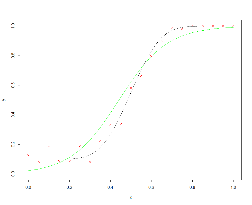
I know for certain that the minimum value of y is 0.1 and the intercept is 0.1. Some observed y values are smaller than 0.1 simply due to random error in measurement. How do I fit a binomial line-of-best fit to this data, accounting for the fact that I know the intercept is 0.1? If I don't account for this, then I could draw the green line, which is clearly wrong.

plot(x, y, ylim = c(0, 1), col = 'red')
abline(h = 0.1, lty = 2)
m <- glm(y ~ x, family = 'binomial')
p <- predict(m, newdata = data.frame(x = x), type = 'response')
lines(x, p, col = 'green')

The line-of-best-fit should be more like the dotted black line, but I don't know how to estimate that.

Answer 1

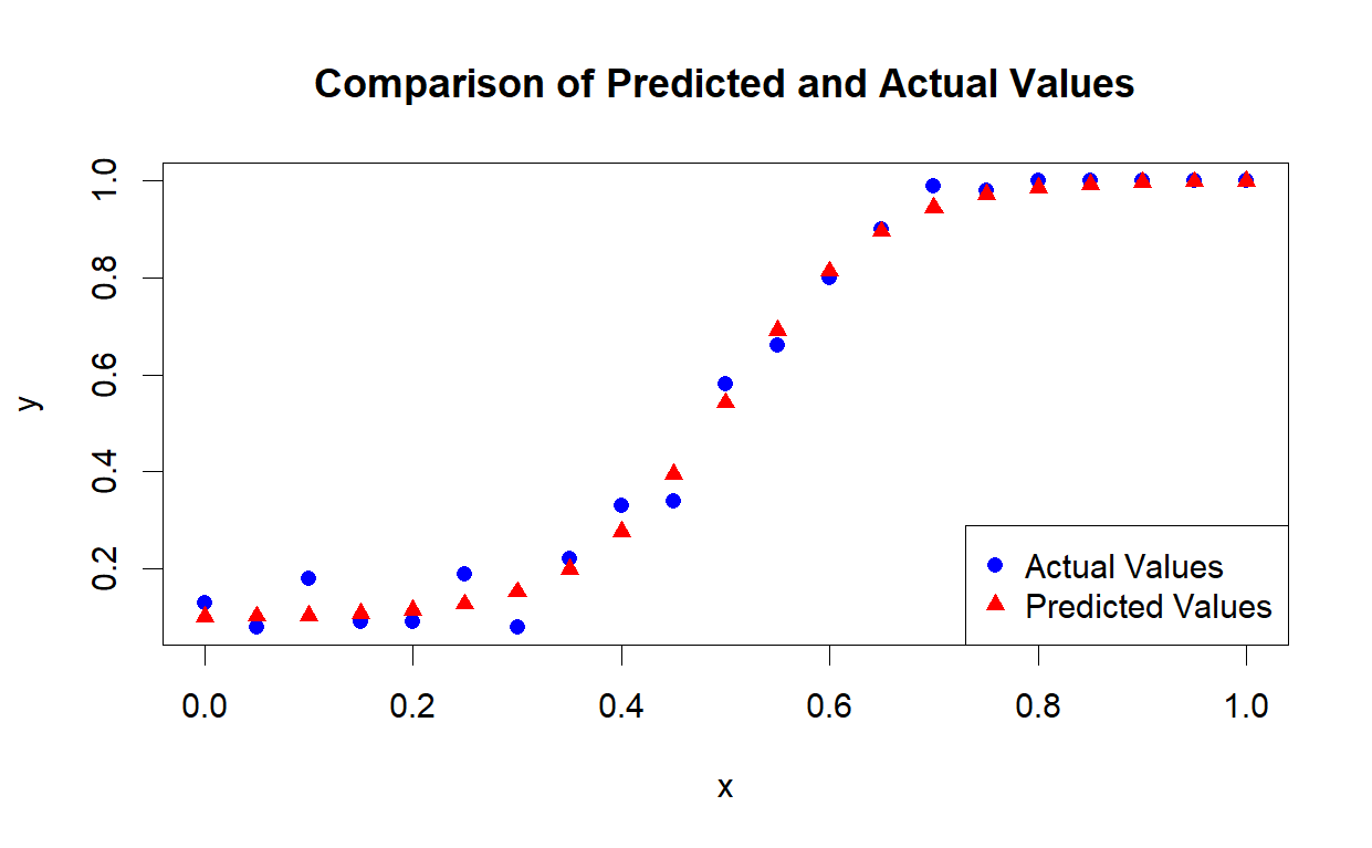
A quick workaround is to use nonlinear least squares estimation and bound the S-shaped curve to the (0.1,1) range.

# estimate the model with adjusted asymptotes
m1 <- nls(y ~ 0.1 + 0.9*exp(a+b*x)/(1 + exp(a+b*x)), 
        start = list(a=0, b = 0))

# predict y
y_predicted = predict(m1, x)

# Plot the actual values with points only
plot(x, y, type = 'p', col = 'blue', pch = 16, xlab = 'x', ylab = 'y', 
     main = 'Comparison of Predicted and Actual Values')

# Add the predicted values with points only
points(x, y_predicted, type = 'p', col = 'red', pch = 17)

# Add a legend to the plot
legend("bottomright", legend=c("Actual Values", "Predicted Values"), 
       col=c("blue", "red"), pch=c(16, 17))

Answer 2

If you want a logistic regression with a pre-specified intercept, you can remove the intercept from the model and replace it by a known offset.

x <- c(1, 0.95, 0.9, 0.85, 0.8, 0.75, 0.7, 0.65, 0.6, 0.55, 0.5, 0.45,
       0.4, 0.35, 0.3, 0.25, 0.2, 0.15, 0.1, 0.05, 0)
y <- c(1, 1, 1, 1, 1, 0.98, 0.99, 0.9, 0.8, 0.66, 0.58, 0.34, 0.33, 
       0.22, 0.08, 0.19, 0.09, 0.09, 0.18, 0.08, 0.13)
intercept <- rep(0.1, length(x))

m <- glm(y ~ 0 + x + offset(intercept), family=binomial)

That, however, does not give anything like the result you want -- it seems that the model isn't close to a logistic regression. So you might actually need to use the nls approach.