A practical example for MCMC

Question

I was going through some lectures related to MCMC. However, I don't find a good example of how it is used. Can anyone give me a concrete example. All I can see that is they run a Markov chain and say that its stationary distribution is the desired distribution.

I want a good example where the desired distribution is hard to sample from. So we create a Markov chain. I want to know how to select the transition matrix so that its stationary distribution, of the Markov chain is the target distribution Thanks

Answer 1

A good example of a distribution that is hard to sample from is the Hard-Core model, see this page for an overview:

http://www.mathematik.uni-ulm.de/stochastik/lehre/ss06/markov/skript_engl/node34.html

This model defines a distribution over $n \times n$ grids for some fixed $n$, where at each point in the grid you can have a value of either one or zero. In order for a grid to be admissible under the hard-core model, no two adjacent points on the grid can both have a value of 1.

The image below shows an example admissible configuration for an $8 \times 8$ grid under the hard-core model. In this image ones are shown as black dots, and zeros as white. Note that not two black dots are adjacent.

I believe the inspiration for this model comes from physics, you can think of each position in the grid being a particle, and the value at that position representing electric charge, or spin.

We want to sample uniformly from the population of admissible grids, that is if $E$ is the set of admissible grids, we want to sample $e \in E$ such that

$ p(e) = \frac{1}{|E|} $

where $|E|$ is the number of all possible admissible configurations.

Already this presents a challenge, given that we are considering $n \times n$ grids, how can we determine $|E|$ the number of admissible grids?

One of the nice things about MCMC, is that it allows you to sample from distributions where the normalizing constant is difficult or impossible to evaluate.

I'll let you read the paper on the details of of how to implement MCMC for this problem, but it is relatively straightforward.

Answer 2

I think the best example I can give you is this:

A Markov Chain Monte Carlo example by Murali Haran

Which includes some useful code in R.

I think that I could reproduce the article here, but it makes no sense.

Answer 3

Another daunting issue in statistics. The question is old, but the introductory examples on-line are hard to come by. So let me simplify two great examples just in case someone following the Markov random walk of PageRank lands here befuddled by MCMC, and full of anticipation for an easy to follow answer. How likely? That could be a follow-up question.

FIRST EXAMPLE:

The post recreates a standard normal distribution $N(0,1)$ using the Metropolis - Hastings algorithm. Far from a challenging case but a good one to dissect. I have collected the code from the post here for convenience and for annotations.

The difficulty is in realizing that after going through all the mechanical steps, there is just one magical trick: the binary decision of accepting or rejecting a proposed value.

It's good to keep in mind that what we want is to generate a bunch of values ($x$) that when plotted on a histogram look like a bell curve, centered (mean) at $0$ and with a standard deviation (sd) of $~ 1$. The problem is that we don't have predetermined parameters; that would be too easy, simply running something along the lines of rnorm(10000).

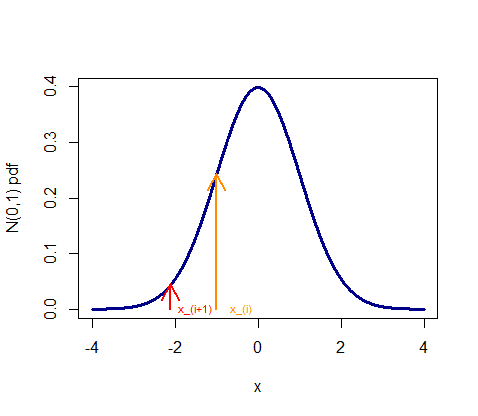
We do so by taking tiny (or larger, it won't change the results too much) random stochastic steps through the use of pseudorandom number generators. In the example, the magnitude of the step is set by eps, which determines the $\epsilon$, or size of the step to the left or to the right from the previous accepted value ($x_i$). This will be the starting line in the process that generates a new proposed value to fill in the next "link" of the "chain", $x_{i+1}$. OK, I'm talking about generating runif(1, - eps, eps) to either subtract or add to $x_i$.

Every proposed value would thus differ from the prior value in a random fashion, and within the boundaries of [- eps,+ eps].

Enter the Markov kernel. We need to assess the probability of transitioning to the new proposed value somehow, much like in a transition Markov matrix on a given state at time $i$ tells about the probability of the new state at time $i + 1$. If in doubt go here, or ask the grandma who's been paying attention to all the "How would you explain quantum physics to your nanna?" type of questions (don't the matrices look nice? ;-) ).

To get this probability of acceptance into the bouquet of culled values, we simply compare the height of the $N(0,1)$ density at the proposed new value ($x_{i+1}$) to the previous (already accepted value), ($x_{i}$), just like this:

And we take the ratio of both values: min(1, dnorm(candidate_value)/dnorm(x)). Since we want a probability, the resultant calculation cannot go over $1$, which occurs whenever the $N(0,1)$ $pdf$ at $x_{i+1}$ (candidate value) is greater than at $x_i$, amounting to automatic acceptance of the proposed value, and explaining the min(1, ...) part of the code. Otherwise, the closer the dnorm value of the proposed value is to the previous value, the higher the odds of it being accepted.

So we do have a probability of acceptance, but we need to make a binary decision (accept the new proposed value, or reject it). And here comes the magic trick: if the probability calculated as min(1, dnorm(candidate_value)/dnorm(x)) is greater than a runif(1) uniform draw from $0$ to $1$ (as close as it gets to a coin toss for a continuous value), we accept, and fill in the x[i+1] entry of the chain with the proposed value; otherwise, we fill it in with a repeat of the previous value, x[i]... The idea would be, better two of the same than one too far away into the tails.

We do this thousands of times and we collect all these values (only the accepted and repeated values), and when we plot the histogram, we get a nice normal curve with a sd close to $1$, and centered at $0$.

Just one final point: Where do we start? Probably not to relevant, but in the simulation, we fill in the first value as $0$, x = 0; vec[1] = x before looping through all the rest of iterations, and let the process follow its course.

SECOND EXAMPLE:

This is more exciting, and makes reference to estimating the parameters of a linear regression curve by calculating log likelihoods for random parameters given a dataset. However, the exegesis of the code lines is built in the condensed simulation saved here, following very similar steps to the first example.

Answer 4

This Youtube video is a really nice visualization of a simple problem that's solved using MCMC.

The distribution of interest is the posterior distribution over possible slopes and intercepts in a linear regression (upper-right panel). Some combinations of slopes and intercepts are very probable (i.e. they have a high likelihood of producing the observed data points and are consistent with our a priori expectations), so they should be sampled frequently. Other combinations are improbable (e.g. if they correspond to a blue line that doesn't go through the cloud of data points), and should be sampled less often.

The big panel in the lower-left shows the path taken by the Markov chain through a two-dimensional space of slopes and intercepts. The histograms show one-dimensional summaries of the chain's progress so far. Once the chain has run long enough, we have very good estimates of the distributions for possible values of the slope and intercept.

In this case, MCMC is overkill, but there are some problems where a solution is hard to write down and it makes a lot of sense to explore the possibilities with a Markov chain rather than trying to solve it directly.