8
$\begingroup$

I'm trying to think through whether the regression

$y = a + b (x/y)$

Is problematic at all. It's not colinearity, because there's no linear relation? But, as $y$ increases, then $bx$ would tend to decrease, so I'm suspicious. Is there a problem here? It's just a regression of $y^2$ on $x$, right?

The real regression in question here is:

$$ \text{Days Attended} = a + b (\text{Incident Count/Days Attended}) $$

where an incident can only occur on a day attended.

$\endgroup$
4
  • 3
    $\begingroup$ Welcome to Cross Validated! How do you figure it is a regression of $y^2$ on $x?$ $\endgroup$
    – Dave
    Commented Sep 27 at 2:25
  • 3
    $\begingroup$ It is likely that this problem can be handled better using some kind of count regression. To aid in our guidance, can you please tell us more about the experimental relationship between incident count and days attended (e.g., is it 0-1 incidents each day attended or can there be more than one incident on a given day attended, etc.). $\endgroup$
    – Ben
    Commented Sep 27 at 3:32
  • $\begingroup$ I agree with @Ben. I'm not sure if there is anything intrinsically wrong with this, but I don't think it's the best approach here, and would like to know more about the data. $\endgroup$
    – Peter Flom
    Commented Sep 27 at 9:24
  • $\begingroup$ You seem to be reversing the natural roles of the variables, as if you conceive of days attended as an uncertain value that depends on an incident count measured with no appreciable error. Is that reasonable? $\endgroup$
    – whuber
    Commented Oct 2 at 19:15

2 Answers 2

10
$\begingroup$

You can get situations where variables end up on both sides of the equation. A good example are the plots used in estimating the parameters of the Michaelis Menten equation.

$$y = \frac{\theta_1x}{\theta_2+x}$$

This is often plotted with some transformed expressions for the horizontal and vertical axes, to linearize the relationship, and you can get variables ending up at both sides of the equation like:

  • Eadie Hofstee plot $$y = a + b \frac{y}{x}$$ with $a = \theta_1$ and $b = -\theta_2$

  • Hanes Woolf plot $$\frac{x}{y} = a + b x$$ with $a = \theta_2/\theta_1$ and $b = 1/\theta_1$


This approach was done because linear functions were easier to estimate (and often done visually instead of by computation) than non-linear functions. Nowadays one would just estimate the parameters based on a non-linear fitting approach.

The problem in general with these approaches, is that the propagation of errors is not obvious. This makes that the estimate is not efficient (has a larger standard error) because it gives wrong weights to different data points. In addition, it is also difficult to give an estimate for the standard error.

The problem in your specific case, is that there is no clear expression for the theoretical background of the equation and information about the sort of errors is completely absent. Do the variables in your situation have some causal relationship like one is independent and the other is dependent? What is the mechanism behind the relationship between these two variables? Possibly you might have originally a quadratic relationship like

$$\text{Incident Count} = - \frac{a}{b}\text{Days Attended} + \frac{1}{b} \text{Days Attended}^2$$


If I am making some assumptions and trying to reverse engineer where your equation comes from, then I get to:

The second derivative would be

$$\Delta \text{Incident Count} = \frac{1}{b} \left(-a + 2 \text{Days Attended}\right)$$

And this would be a model for a situation where the incident count increases every attended day where the increase is linearly increasing. The next day, 2/b more increase in incidents is expected.

You could use this in a Poisson regression where the incident count is Poisson distributed with a rate that is a quadratic function of the number of days attended. It is tricky however, because the incidents might not be random independent events like a Poisson process. So a description of the mechanism that creates the data is useful pin down more exactly what sort of regression is most appropriate. Don't just start using Poisson regression because the internet told you to use it.


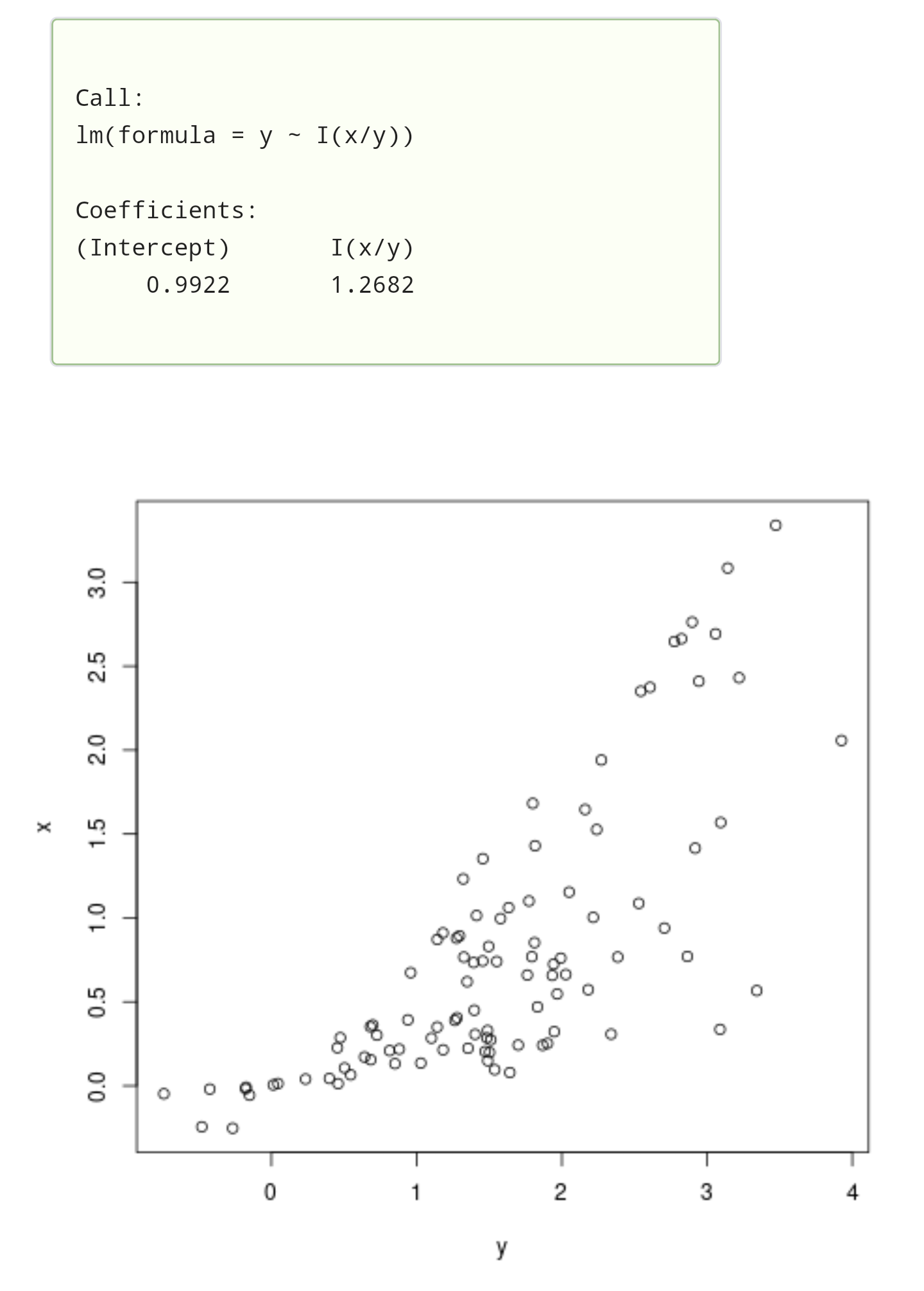
A straightforward example in R where your regression is perfectly fine is when the data would be generated like below (with an unobserved variable $z$ that is in the original linear model, but we happen to observe $z \cdot y$ instead).

It is not clear whether your data is like that, but it demonstrates that there is not anything against your regression y ~ x/y in principle.

set.seed(1) 
a = 1; b = 1
n = 100
noise = rnorm(n)
z = runif(n)
y = a + b*z + noise
x = y*z
plot(y,x)
lm(y ~ I(x/y))

example

$\endgroup$
2
  • 1
    $\begingroup$ off-topic question: how did you generate the output interface as colored? Also, (+1) it's nice to see answers resorting to plots of biochemistry, which at least I was not aware of. $\endgroup$ Commented Sep 27 at 12:46
  • 2
    $\begingroup$ @User1865345 I often use an online R compiler to generate images rdrr.io/snippets $\endgroup$ Commented Sep 27 at 14:08
8
$\begingroup$

I'm trying to think through whether the regression

y=a+b(x/y)

The root of your problem is this is not a correctly expressed regression model, since it leaves something out, and the omission is critical.

In your data, y does not equal $a + b(x/y)$ for any choices of $a$ and $b$, not at every point $(x_i,y_i)$ - and perhaps, not at any point. If it did, you would not need regression at all.

When you try to multiply through by $y$, you do it incorrectly as it stands if you multiply your "equation" through by $y$ and combine terms, you get $y^2-ay$ on the left hand side and $bx$ on the right, but even with that fix, you cannot hope to correctly identify what's going on until you deal with the missing error term.

Your original equation should be (say)

$$y_i = a + b(x_i/y_i) + \varepsilon_i, \qquad i=1,2,\ldots,n$$

for some $\varepsilon_i$, which we have yet to specify the behavior of (assuming independence and zero mean, ideally, you still need its distribution and variance). The problem is still that you have $y$ on both sides, which will cause a number of problems.

If you multiply through by $y_i$ you get:

$$y_i^2 = a y_i + b x_i + \varepsilon_i y_i, \qquad i=1,2,\ldots,n$$

and - while we could again subtract $a y_i$ from both sides and manipulate it - now $y_i$ is also entangled with the error term, and that we can't just "take over to the left hand side".

If we start with the "corrected" version of multiplying through your incomplete equation by "y" and then put an error term on it, we would have:

$$y_i^2 = a y_i + b x_i + \eta_i , \qquad i=1,2,\ldots,n$$

This has some promise, but it's a different model to the one we wrote with an error of $\varepsilon_i y_i$.

This one we can take a little further, manipulating as follows:

$$y_i^2 - a y_i = b x_i + \eta_i$$ (suppressing the $i=...$ for now)

$$y_i^2 - a y_i + \frac{a^2}{4} = \frac{a^2}{4} + b x_i + \eta_i$$

$$(y_i- \frac{a}{2})^2 = \frac{a^2}{4} + b x_i + \eta_i$$

The problem now is that we have a parameter on the left hand side which we require on the right. If $y_i-\frac{a}{2}$ was sure to be non-negative, we could continue:

$$y_i = \frac{a}{2} + \sqrt{\frac{a^2}{4} + b x_i + \eta_i}$$

which does seem to be an improvement, but the problem is this non-linear equation has the error term inside the square root, which entangles it with the predictor and parameters.

You might consider yet another possibility, moving even further astray:

$$y_i = \frac{a}{2} + \sqrt{\frac{a^2}{4} + b x_i} + \zeta_i$$

Now if we assume that the $\zeta_i$ errors are say independent with constant variance, this is a nonlinear regression equation, which you could fit (say by least squares), but we've had to make multiple compromises to get to it, including restricting the possible values of $a$ (in a way that - problematically - depends on the data), and changing the form of the error term. The resulting problem is that it won't get you back to something like what you started with, as we see if we try to reverse the operations:

$$(y_i - \frac{a}{2})^2 = {\frac{a^2}{4} + b x_i} +2\sqrt{\frac{a^2}{4} + b x_i}\zeta_i+ \zeta_i^2$$

$$y_i^2 - a y_i + \frac{a^2}{4} = {\frac{a^2}{4} + b x_i} +2\sqrt{\frac{a^2}{4} + b x_i}\zeta_i+ \zeta_i^2$$

$$y_i^2 = a y_i + b x_i +2\sqrt{\frac{a^2}{4} + b x_i}\zeta_i+ \zeta_i^2$$

$$y_i = a + b \frac{x_i}{y_i} +\frac{ 2\sqrt{\frac{a^2}{4} + b x_i}\zeta_i+ \zeta_i^2}{y_i}$$

so the nonlinear regression is not at all like the original model with an additive error. The error is now entangled with the predictor and the response.

It's not clear to me that any of these models are actually sensible.

$\endgroup$
2
  • 1
    $\begingroup$ +1. But I suspect what the OP really wants to formulate would be the equivalent of $x=(y^2 - ay)/b + \varepsilon:$ that is, a quadratic model that reverses the roles of explanatory and response variables. $\endgroup$
    – whuber
    Commented Oct 2 at 19:17
  • 1
    $\begingroup$ Ah, given what the variables represent, that makes somewhat more sense. $\endgroup$
    – Glen_b
    Commented Oct 2 at 21:57

Your Answer

By clicking “Post Your Answer”, you agree to our terms of service and acknowledge you have read our privacy policy.

Not the answer you're looking for? Browse other questions tagged or ask your own question.