Can we calculate population mean response from GLMM by averaging over random effects?

Question

I am trying to understand how we can estimate the effect of a covariate on population mean response when we have fitted a generalised linear mixed model with non-linear link function to the data. I refer to section 13.3 of Fitzmaurice et al. (2011) for our discussion.

For example, consider the logistic regression model with a randomly varying intercept, $$logit\{E( Y_i|b_i )\} = X_i\beta^* + b_i,$$ where $b_i \sim {N(0, \sigma_b ^2)}$.

Let $e^{X_i\beta^* \ + \ b_i} = c$.

The implied model for marginal mean or marginal probability of success is

$$ E(Y_i) = \int_{-\infty}^{\infty}{\frac{c}{(1 + c)\sqrt{2\pi\sigma_b^2}}}e^{\frac{-b_i^2}{2\sigma^2_b}}db_i $$

In the above integral, the notion of $b_i$ being a random variable is clear.

[the above] expression cannot be evaluated in closed-form. $\dots$From a purely probabilistic point of view, generalized linear mixed models might appear to have a distinct advantage over marginal models since the marginal distribution of $Y_i$, the target of inference for marginal models, can, in principle, be derived from the generalized linear mixed effects model by averaging over the distribution of the random effects.

Because the authors did not explicitly mention how to perform such averaging, I referred to the section 16.3 of Molenberghs and Verbeke (2005) for more information:

Again, numerical integration methods can be used, but it is often much easier to use numerical averaging by sampling a large number $M$ of random-effects vectors $b_i$ from their fitted distribution $N(0, \hat{D})$, and to estimate ${E}[Y_i]$ by

$$ \hat{E}(Y_i) = \frac{1}{M} \sum_{1}^{M}{\frac{exp(X_i\hat{\beta^*} + b_i)}{1 + exp(X_i\hat{\beta^*} + b_i)}} $$

It seems to me that this estimation procedure does not hold on the notion that $b_i$ is a random variable because it assigns equal weights ($\frac{1}{M}$) to all the sampled values of $b_i$. Won't the following expression be more helpful?

$$ \hat{E}(Y_i) = \sum_{1}^{M}{\frac{exp(X_i\hat{\beta^*} + b_i)}{1 + exp(X_i\hat{\beta^*} + b_i)}\cdot P(b_i)} $$

Whether or not the above expression is helpful, would the calculation suggested by Molenberghs and Verbeke be similar to the estimated marginal means computed by emmeans for a GLMM?

---

Fitzmaurice, G. M., Laird, N. M., & Ware, J. H. (2012). Applied longitudinal analysis. John Wiley & Sons.

Models for Discrete Longitudinal Data. (2005). In Springer Series in Statistics. Springer-Verlag. https://doi.org/10.1007/0-387-28980-1

Answer 1

Working with just the means on the logit scale (equivalent to averaging on the logit scale, which I think is what emmeans currently does - but who knows, maybe they'll add options in the future to do additional things) doesn't give you the marginal (aka population) mean because of the non-linear nature of the link function, so indeed the integration mentioned is what one should do if that's what one wants. We could of course debate, whether you should also account for the uncertainty about $\hat{D}$.

Obviously, in your simple example with just a random intercept, it's still pretty straightforward to implement a analytical or numeric integration. The Monte-Carlo approach mentioned by Molenberghs and Verbeke (2005) seems more generally applicable. You're notation with $P(b_i)$ seems confusing to wrong me, $1/M$ is exactly the right term here.

This all becomes a lot easier, if you fit this a Bayesian model with MCMC. There, it gets a lot easier to directly ask for the predictive distribution for new patients with particular characteristics. Working through this with MCMC samples tends to be really helpful for understanding what is going on. One can do this rather easily e.g. with the brms R package. The model would just look like fit1 <- brm(y ~ (1|subject) + x, family = bernoulli(link = "logit")) followed by either the direct implementation via like posterior_epred(fit1, newdata = my_new_data_with_new_subject_ids, allow_new_levels=TRUE, sample_new_levels="gaussian") or doing your own calculations via posterior::as_draws_df(fit1) or my_new_data_with_new_subject_ids %>% tidybayes::add_epred_draws() etc.

Answer 2

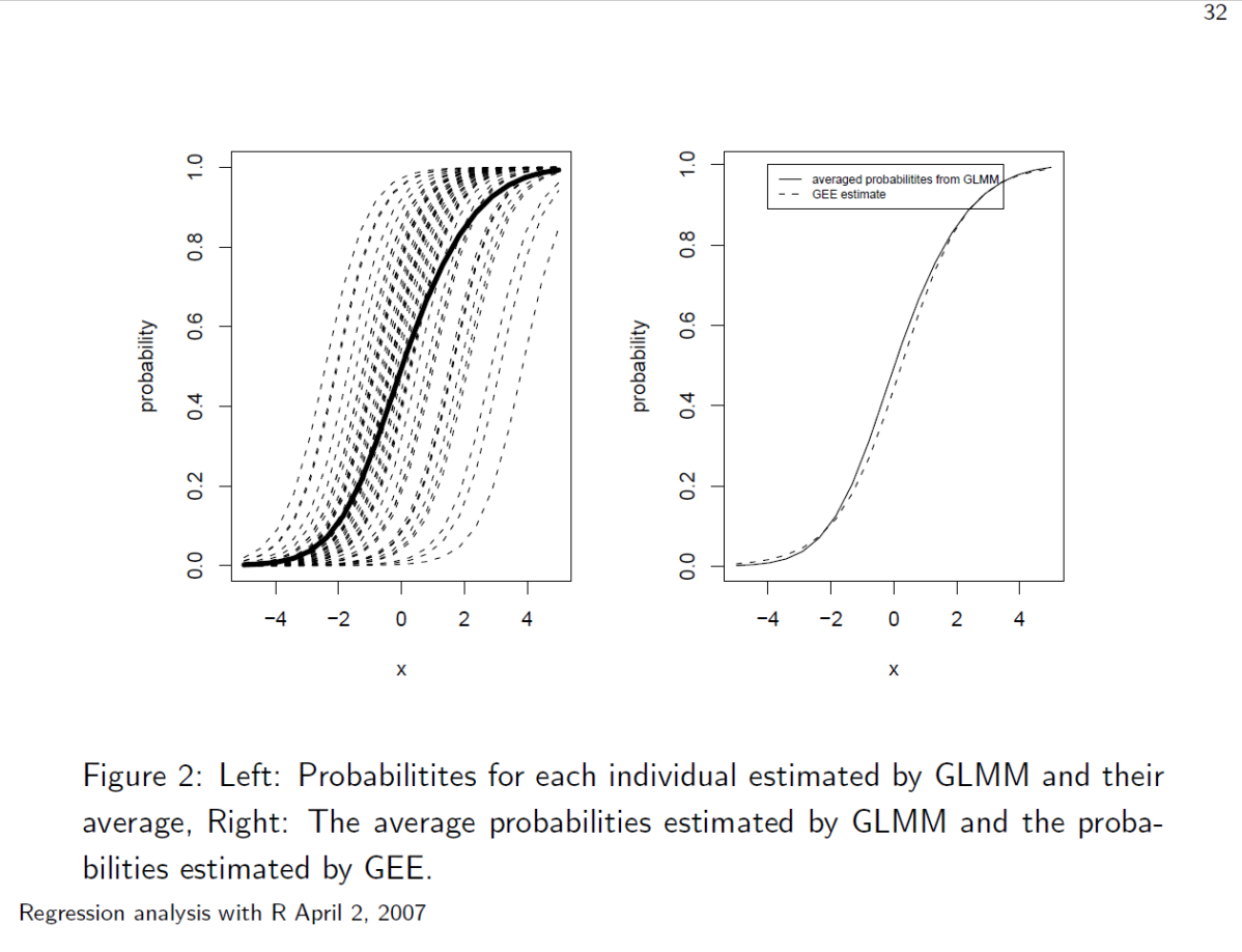
I am not sure about those formulae, and leave that to better mathematicians than I. But yes, averaging over random intercepts or slopes will not produce the population average in the case of GLM's. To find that, people often resort to Generalised Estimating Equations, while the GLMMs will be ever so slightly off. The lecture slide below from Højsgaard and Ulrich Halekoh, 2007, plots this out in detail in the right hand plot. Note, for normal regressions the estimates for both methods are the same, and you can use either.

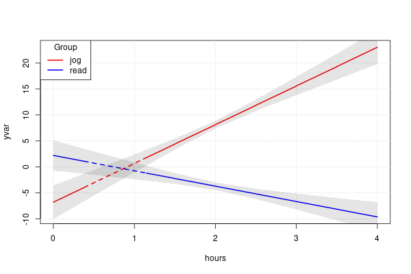
Also, note, the emmeans package only gives marginal estimates in a sense of the word. It's not really a true population mean, except under rare cases. What the package does is effect (deviance) code the contrast matrix so that the intercept is the mean between the groups' means. If your group sizes are equal that will be the population/marginal mean, but it often is not. So, it does help when you do post-estimation modelling, or plotting, to produce the plot below to be able to straight forwardly say "the difference between jogging and reading is X (averaged over all the various categorical variables)", instead of "the average difference for a tall, short sighted, boy, from country A, compared to a short, far sighted, ..."

But still that intercept is not quite the population average.