I have a question about the Kullback-Leibler divergence.
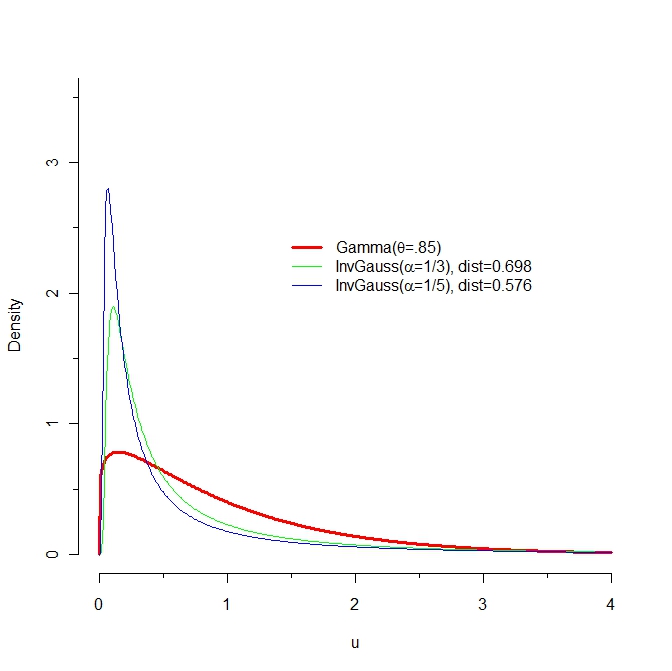
Can someone explain why the "distance" between the blue density and the "red" density is smaller than the distance between the "green" curve and the "red" one?
I have a question about the Kullback-Leibler divergence.
Can someone explain why the "distance" between the blue density and the "red" density is smaller than the distance between the "green" curve and the "red" one?

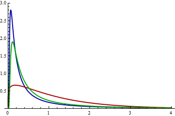
Because I compute slightly different values of the KL divergence than reported here, let's start with my attempt at reproducing the graphs of these PDFs:
The KL distance from $F$ to $G$ is the expectation, under the probability law $F$, of the difference in logarithms of their PDFs. Let us therefore look closely at the log PDFs. The values near 0 matter a lot, so let's examine them. The next figure plots the log PDFs in the region from $x=0$ to $x=0.10$:
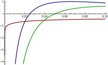
Mathematica computes that KL(red, blue) = 0.574461 and KL(red, green) = 0.641924. In the graph it is clear that between 0 and 0.02, approximately, log(green) differs far more from log(red) than does log(blue). Moreover, in this range there is still substantially large probability density for red: its logarithm is greater than -1 (so the density is greater than about 1/2).
Take a look at the differences in logarithms. Now the blue curve is the difference log(red) - log(blue) and the green curve is log(red) - log(green). The KL divergences (w.r.t. red) are the expectations (according to the red pdf) of these functions.
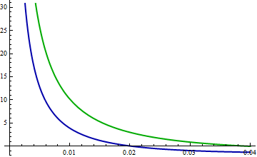
(Note the change in horizontal scale, which now focuses more closely near 0.)
Very roughly, it looks like a typical vertical distance between these curves is around 10 over the interval from 0 to 0.02, while a typical value for the red pdf is about 1/2. Thus, this interval alone should add about 10 * 0.02 /2 = 0.1 to the KL divergences. This just about explains the difference of .067. Yes, it's true that the blue logarithms are further away than the green logs for larger horizontal values, but the differences are not as extreme and the red PDF decays quickly.
In brief, extreme differences in the left tails of the blue and green distributions, for values between 0 and 0.02, explain why KL(red, green) exceeds KL(red, blue).
Incidentally, KL(blue, red) = 0.454776 and KL(green, red) = 0.254469.
Specify the distributions
red = GammaDistribution[1/.85, 1];
green = InverseGaussianDistribution[1, 1/3.];
blue = InverseGaussianDistribution[1, 1/5.];
Compute KL
Clear[kl];
(* Numeric integation between specified endpoints. *)
kl[pF_, qF_, l_, u_] := Module[{p, q},
   p[x_] := PDF[pF, x];
   q[x_] := PDF[qF, x];
   NIntegrate[p[x] (Log[p[x]] - Log[q[x]]), {x, l, u},
    Method -> "LocalAdaptive"]
   ];
(* Integration over the entire domain. *)
kl[pF_, qF_] := Module[{p, q},
   p[x_] := PDF[pF, x];
   q[x_] := PDF[qF, x];
   Integrate[p[x] (Log[p[x]] - Log[q[x]]), {x, 0, \[Infinity]}]
   ];

kl[red, blue]
kl[red, green]
kl[blue, red, 0, \[Infinity]]
kl[green, red, 0, \[Infinity]]
Make the plots
Clear[plot];
plot[{f_, u_, r_}] :=
  Plot[Evaluate[f[#, x] & /@ {blue, red, green}], {x, 0, u},
   PlotStyle -> {{Thick, Darker[Blue]}, {Thick, Darker[Red]},
     {Thick, Darker[Green]}},
   PlotRange -> r,
   Exclusions -> {0},
   ImageSize -> 400
   ];
Table[
  plot[f], {f, {{PDF, 4, {Full, {0, 3}}}, {Log[PDF[##]] &,
     0.1, {Full, Automatic}}}}
  ] // TableForm

Plot[{Log[PDF[red, x]] - Log[PDF[blue, x]],
  Log[PDF[red, x]] - Log[PDF[green, x]]}, {x, 0, 0.04},
 PlotRange -> {Full, Automatic},
 PlotStyle -> {{Thick, Darker[Blue]}, {Thick, Darker[Green]}}]
KL divergence measures how difficult it is to fake one distribution with another one. Assume that you draw an i.i.d. sample of size $n$ from the red distribution and that $n$ is large. It may happen that the empirical distribution of this sample mimicks the blue distribution. This is rare but this may happen... albeit with a probability which is vanishingly small, and which behaves like $\mathrm{e}^{-nH}$. The exponent $H$ is the KL divergence of the blue distribution with respect to the red one.
Having said that, I wonder why your KL divergences are ranked in the order you say they are.