Let's assume we restrict consideration to symmetric distributions where the mean and variance are finite (so the Cauchy, for example, is excluded from consideration).
Further, I'm going to limit myself initially to continuous unimodal cases, and indeed mostly to 'nice' situations (though I might come back later and discuss some other cases).
The relative variance depends on sample size. It's common to discuss the ratio of ($n$ times the) the asymptotic variances, but we should keep in mind that at smaller sample sizes the situation will be somewhat different. (The median sometimes does noticeably better or worse than its asymptotic behaviour would suggest. For example, at the normal with $n=3$ it has an efficiency of about 74% rather than 63%. The asymptotic behavior is generally a good guide at quite moderate sample sizes, though.)
The asymptotics are fairly easy to deal with:
Mean: $n\times$ variance = $\sigma^2$.
Median: $n\times$ variance = $\frac{1}{[4f(m)^2]}$ where $f(m)$ is the height of the density at the median.
So if $f(m)>\frac{1}{2\sigma}$, the median will be asymptotically more efficient.
[In the normal case, $f(m)= \frac{1}{\sqrt{2\pi}\sigma}$, so $\frac{1}{[4f(m)^2]}=\frac{\pi\sigma^2}{2}$, whence the asymptotic relative efficiency of $2/\pi$)]
We can see that the variance of the median will depend on the behaviour of the density very near the center, while the variance of the mean depends on the variance of the original distribution (which in some sense is affected by the density everywhere, and in particular, more by the way it behaves further away from the center)
Which is to say, while the median is less affected by outliers than the mean, and we often see that it has lower variance than the mean when the distribution is heavy tailed (which does produce more outliers), what really drives the performance of the median is inliers. It often happens that (for a fixed variance) there's a tendency for the two to go together.
That is, broadly speaking, as the tail gets heavier, there's a tendency for (at a fixed value of $\sigma^2$) the distribution to get "peakier" at the same time (more kurtotic, in a loose sense). This is not, however, a certain thing - it tends to be the case across a broad range of commonly considered densities, but it doesn't always hold. When it does hold, the variance of the median will reduce (because the distribution has more probability in the immediate neighborhood of the median), while the variance of the mean is held constant (because we fixed $\sigma^2$).
So across a variety of common cases the median will often tend to do "better" than the mean when the tail is heavy, (but we must keep in mind that it's relatively easy to construct counterexamples). So we can consider a few cases, which can show us what we often see, but we shouldn't read too much into them, because heavier tail doesn't universally go with higher peak.
We know the median is about 63.7% as efficient (for $n$ large) as the mean at the normal.
What about, say a logistic distribution, which like the normal is approximately parabolic about the center, but has heavier tails (as $x$ becomes large, they become exponential).
If we take the scale parameter to be 1, the logistic has variance $\pi^2/3$ and height at the median of 1/4, so $\frac{1}{4f(m)^2}=4$. The ratio of variances is then $\pi^2/12\approx 0.82$ so in large samples, the median is roughly 82% as efficient as the mean.
Let's consider two other densities with exponential-like tails, but different peakedness.
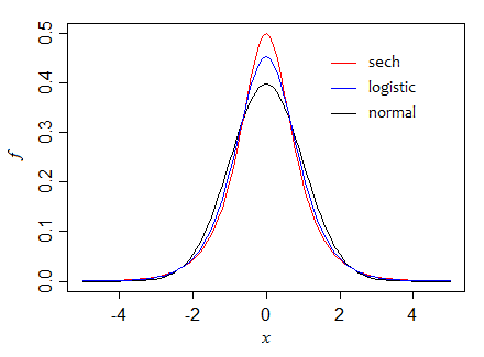
First, the hyperbolic secant ($\text{sech}$) distribution, for which the standard form has variance 1 and height at the center of $\frac{1}{2}$, so the ratio of asymptotic variances is 1 (the two are equally efficient in large samples). However, in small samples the mean is more efficient (its variance is about 95% of that for the median when $n=5$, for example).
Here we can see how, as we progress through those three densities (holding variance constant), that the height at the median increases:

Can we make it go still higher? Indeed we can. Consider, for example, the double exponential. The standard form has variance 2, and the height at the median is $\frac{1}{2}$ (so if we scale to unit variance as in the diagram, the peak is at $\frac{1}{\sqrt{2}}$, just above 0.7). The asymptotic variance of the median is half that of the mean.
If we make the distribution peakier still for a given variance, (perhaps by making the tail heavier than exponential), the median can be far more efficient (relatively speaking) still. There's really no limit to how high that peak can go.
If we had instead used examples from say the t-distributions, broadly similar effects would be seen, but the progression would be different; the crossover point is a little below $\nu=5$ df (actually around 4.68) -- for smaller df the median is more efficient, for large df the mean is.
...
At finite sample sizes, it's sometimes possible to compute the variance of the distribution of the median explicitly. Where that's not feasible - or even just inconvenient - we can use simulation to compute the variance of the median (or the ratio of the variance*) across random samples drawn from the distribution (which is what I did to get the small sample figures above).
* Even though we often don't actually need the variance of the mean, since we can compute it if we know the variance of the distribution, it may be more computationally efficient to do so, since it acts like a control variate (the mean and median are often quite correlated).
