Return to Revisions

I'm assuming that a model which was fitted using the Error() function within aov() won't work when using in plot() because you will get more than one error stratum from which you can choose. Now you could use the proj() function which will give you the residuals for each error stratum in a way that allows you to extract them more easily. I found some information here.

Edit start

More information regarding multistratum models and the proj() function is given in Venables and Ripley, page 284 (but start from page 281): Residuals in multistratum analyses: Projections. In the second sentence they write (I highlighted in bold):

Thus fitted(oats.aov[[4]]) and resid(oats.aov[[4]]) are vectors of length 54 representing fitted values and residuals from the last stratum, based on 54 orthonormal linear functions of the original data vector.

For your example that means:

ex.aov.proj <- proj(ex.aov)

# Check number of strata 
summary(ex.aov.proj)

# Check for normality by using last error stratum
qqnorm(ex.aov.proj[[9]][, "Residuals"])
# Check for heteroscedasticity by using last error stratum
plot(ex.aov.proj[[9]][, "Residuals"])

However, this will also lead into plots which I cannot fully interpret (especially the second one).

In their case, the last stratum was the Within stratum. Since your model cannot estimate this (presumably due to your error term), I am not sure if simply using your last stratum is valid.

Hopefully someone else can clarify.

Edit end

My alternative suggestion:

First, I changed your dataset slightly and set a seed to make it reproducible (might be handy for some problems you have in the future):

# Set seed to make it reproducible
set.seed(12)

# I changed the names of your variables to make them easier to remember
# I also deleted a few nested `rep()` commands. Have a look at the `each=` argument.
subj <- sort(factor(rep(1:20,8)))
x1 <- rep(c('A','B'),80)
x2 <- rep(c('A','B'),20,each=2)
x3 <- rep(c('A','B'),10, each=4)
outcome <- rnorm(80,10,2)

d3 <- data.frame(outcome,subj,x1,x2,x3)

Second, I used a linear mixed-effects model instead since you have repeated measures and hence a random term you can use:

require(lme4)
# I specified `subj` as random term to account for the repeated measurements on subject.
m.lmer<-lmer(outcome ~ x1*x2*x3 + (1|subj), data = d3)
summary(m.lmer)

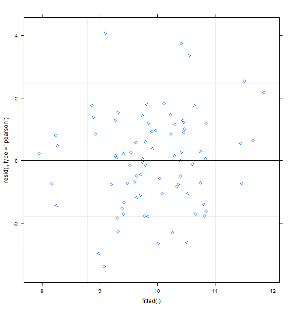
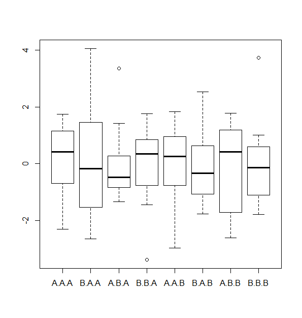
# Check for heteroscedasticity
plot(m.lmer)

# or
boxplot(residuals(m.lmer) ~ d3$x1 + d3$x2 + d3$x3)

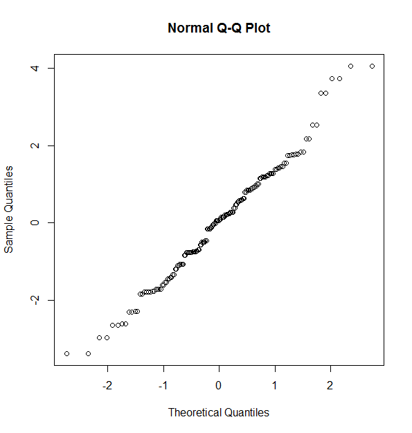
# Check for normality
qqnorm(residuals(m.lmer))

Using the afex package you can also get the fixed effects in ANOVA table format (you can also use the Anova() function from the car package as another option):

require(afex)
mixed(outcome ~ x1*x2*x3 + (1|subj), data = d3, method="LRT")

Fitting 8 (g)lmer() models:
[........]
    Effect df    Chisq p.value
1       x1  1     0.04     .84
2       x2  1     2.53     .11
3       x3  1  7.68 **    .006
4    x1:x2  1  8.34 **    .004
5    x1:x3  1 10.51 **    .001
6    x2:x3  1     0.31     .58
7 x1:x2:x3  1     0.12     .73

Check ?mixed for the various options you can choose. Also regarding mixed models, there is a lot of information here on Cross Validated.