Don't use integers when specifying factors when you use aov() (even if you explicitly changed to a factor). For some reason this will not work well.
So instead of:
p <- sort(rep(1:20,8))
y <- rep(rep(1:2,4),20)
z <- rep(rep(c(1,1,2,2),2),20)
w <- rep(c(1,1,1,1,2,2,2,2),20)
x <- rnorm(160,10,2)

d0 <- data.frame(x,p=factor(p),y=factor(y),z=factor(z),w=factor(w))

ex.aov0<- aov(x ~ y*z*w + Error(p/(y*z*w)), d0)
Edit (to address OP's comment):
You can also keep integers but then you have to make them as.character first and then turn them into a factor:
d1 <- data.frame(x,p=p,y=as.character(y),z=as.character(z),w=as.character(w))
d1$y <- factor(d1$y, levels=c(1,2), labels=c("A","B"))
d1$z <- factor(d1$z, levels=c(1,2), labels=c("A","B"))
d1$w <- factor(d1$w, levels=c(1,2), labels=c("A","B"))

ex.aov1<- aov(x ~ y*z*w + Error(p/(y*z*w)), d1)
Edit end.
use:
# I used "_f" to designate the change to a factor
p <- sort(rep(1:20,8))
y_f <- rep(rep(c("A","B"),4),20)
z_f <- rep(rep(c("A","A","B","B"),2),20)
w_f <- rep(c("A","A","A","A","B","B","B","B"),20)
x <- rnorm(160,10,2)

d2 <- data.frame(x,p,y_f,z_f,w_f)

ex.aov2 <- aov(x ~ y_f * z_f * w_f + Error(p / (y_f * z_f * w_f)), d2)
Now compare: summary(ex.aov0) vs. summary(ex.aov1) vs. summary(ex.aov2)
ex.aov2 will also now give you the error : within part of the output which you didn't get before.
Regarding your plots, why did you choose p:y:z and not y:z:w as these are your independent variables? I am just curious. In any case, if you change it, it will not work:
plot(residuals(ex.aov2[["y_f : z_f : w_f"]]) ~ fitted(ex.aov2[["y_f : z_f : w_f"]]))
However, the reason why aov() objects fitted with the Error() function are not working in plot() commands, I don't know.
My alternative suggestion:
First, I changed your dataset slightly and set a seed to make it reproducible (might be handy for some problems you have in the future):
# Set seed to make it reproducible
set.seed(12)

# I changed the names of your variables to make them easier to remember
# I also deleted a few nested `rep()` commands. Have a look at the `each=` argument.
subj <- sort(rep(1:20,8))
x1 <- rep(c('A','B'),160)
x2 <- rep(c('A','B'),40,each=2)
x3 <- rep(c('A','B'),20, each=4)
outcome <- rnorm(160,10,2)

d3 <- data.frame(outcome,subj,x1,x2,x3)
Second, I used a linear mixed-effects model instead since you have repeated measures and hence a random term you can use:
require(lme4)
# I specified `subj` as random term to account for the repeated measurements on subject.
m.lmer<-lmer(outcome ~ x1*x2*x3 + (1|subj), data = d3)
summary(m.lmer)

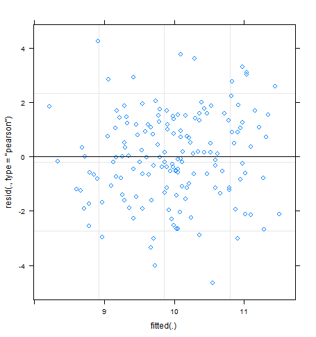
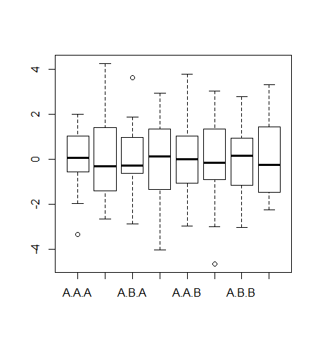
# Check for heteroscedasticity
plot(m.lmer)
# or
boxplot(residuals(m.lmer) ~ d3$x1 + d3$x2 + d3$x3)
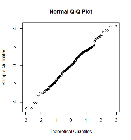
# Check for normality
qqnorm(residuals(m.lmer))
Using the afex package you can also get the fixed effects in ANOVA table format (you can also use the Anova() function from the car package as another option):
require(afex)
mixed(outcome ~ x1*x2*x3 + (1|subj), data = d3, method="LRT")

Fitting 8 (g)lmer() models:
[........]
    Effect df     Chisq p.value
1       x1  1      0.66     .42
2       x2  1      0.22     .64
3       x3  1 21.16 ***  <.0001
4    x1:x2  1    3.40 +     .07
5    x1:x3  1    3.99 *     .05
6    x2:x3  1    2.83 +     .09
7 x1:x2:x3  1      0.00     .97
Check ?mixed for the various options you can choose. Also regarding mixed models, there is a lot of information here on Cross Validated.


