Regarding your plots, I assume that fitting aov() with the Error() function won't work because you will get more than one error stratum.
You can see this with print(ex.aov). Now you could use the proj() function which will give you the residuals
for each error stratum in a way that allows you to extract them more easily.
I found some information here.
print(ex.aov)

ex.aov.proj <- proj(ex.aov)

# Check for normality by using the 5th error stratum as an example since there is no `Error:Within` stratum
qqnorm(ex.aov.proj[[5]][, "Residuals"])
# Check for heteroscedasticity by using the 5th error stratum as an example since there is no `Error:Within` stratum
plot(ex.aov.proj[[5]][, "Residuals"])
However, this will also lead into plots which I cannot fully interpret but I think it has to do with the fact that you don't
have multiple measurements for all factor combinations within p and your error term doesn't allow for an Error:Within stratum. But I am not sure. Does your real dataset have the exact
same structure (inlcuding number of observations)? Hopefully someone else can clarify.
My alternative suggestion:
First, I changed your dataset slightly and set a seed to make it reproducible (might be handy for some problems you have in the future):
# Set seed to make it reproducible
set.seed(12)

# I changed the names of your variables to make them easier to remember
# I also deleted a few nested `rep()` commands. Have a look at the `each=` argument.
subj <- sort(rep(1:20,8))
x1 <- rep(c('A','B'),160)
x2 <- rep(c('A','B'),40,each=2)
x3 <- rep(c('A','B'),20, each=4)
outcome <- rnorm(160,10,2)

d3 <- data.frame(outcome,subj,x1,x2,x3)
Second, I used a linear mixed-effects model instead since you have repeated measures and hence a random term you can use:
require(lme4)
# I specified `subj` as random term to account for the repeated measurements on subject.
m.lmer<-lmer(outcome ~ x1*x2*x3 + (1|subj), data = d3)
summary(m.lmer)

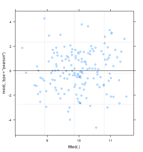
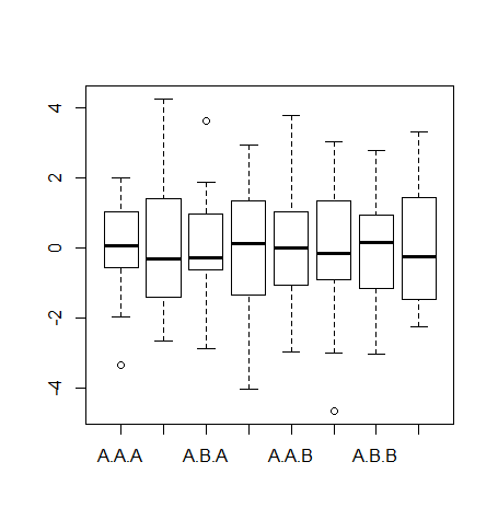
# Check for heteroscedasticity
plot(m.lmer)
# or
boxplot(residuals(m.lmer) ~ d3$x1 + d3$x2 + d3$x3)
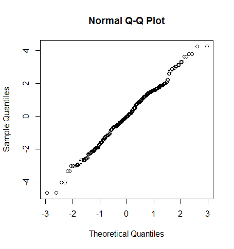
# Check for normality
qqnorm(residuals(m.lmer))
Using the afex package you can also get the fixed effects in ANOVA table format (you can also use the Anova() function from the car package as another option):
require(afex)
mixed(outcome ~ x1*x2*x3 + (1|subj), data = d3, method="LRT")

Fitting 8 (g)lmer() models:
[........]
    Effect df     Chisq p.value
1       x1  1      0.66     .42
2       x2  1      0.22     .64
3       x3  1 21.16 ***  <.0001
4    x1:x2  1    3.40 +     .07
5    x1:x3  1    3.99 *     .05
6    x2:x3  1    2.83 +     .09
7 x1:x2:x3  1      0.00     .97
Check ?mixed for the various options you can choose. Also regarding mixed models, there is a lot of information here on Cross Validated.


