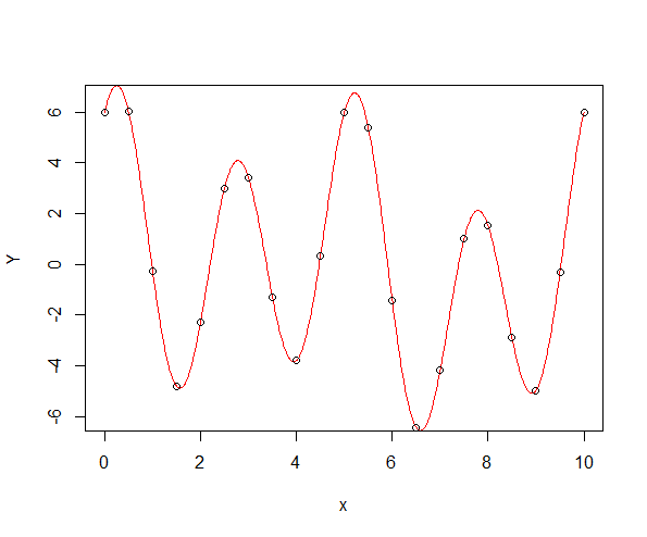
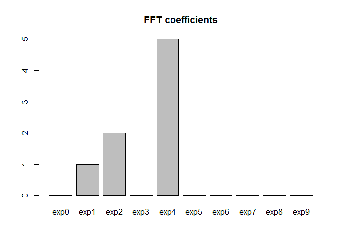
They are strongly related. Your example is not reproducible because you didn't include your data, thus I'll make a new one. First of all, let's create a periodic function:
T <- 10
omega <- 2*pi/T
N <- 21
x <- seq(0, T, len = N)
sum_sines_cosines <- function(x, omega){
    sin(omega*x)+2*cos(2*omega*x)+3*sin(4*omega*x)+4*cos(4*omega*x)
}
Yper <- sum_sines_cosines(x, omega)
Yper[N]-Yper[1] # numerically 0

x2 <- seq(0, T, len = 1000)
Yper2 <- sum_sines_cosines(x2, omega)
plot(x2, Yper2, col = "red", type = "l", xlab = "x", ylab = "Y")
points(x, Yper)
Now, let's create a Fourier basis for regression. Note that, with $N = 2k+1$, it doesn't really make sense to create more than $N-2$ basis functions, i.e., $N-3=2(k-1)$ non-constant sines and cosines, because higher frequency components are aliased on such a grid. For example, a sine of frequency $k\omega$ is indistinguishable from a costant (sine): consider the case of $N=3$, i.e., $k=1$. Anyway, if you want to double check, just change N-2 to N in the snippet below and look at the last two columns: you'll see that they're actually useless (and they create issues for the fit, because the design matrix is now singular).
# Fourier Regression with fda
library(fda)
mybasis <- create.fourier.basis(c(0,T),N-2)
basisMat <- eval.basis(x, mybasis)
FDA_regression <- lm(Yper ~ basisMat-1)
FDA_coef <-coef(FDA_regression)
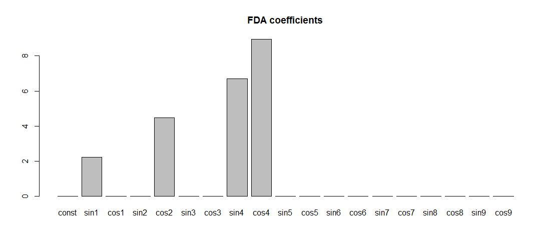
barplot(FDA_coef)
Note that the frequencies are exactly the right ones, but the amplitudes of nonzero components are not (1,2,3,4). The reason is that the fda Fourier basis functions are scaled in a weird way: their maximum value is not 1, as it would be for the usual Fourier basis ${1,\sin{ \omega x},\cos{ \omega x},\dots}$. It's not $\frac{1}{\sqrt \pi}$ either, as it would have been for the orthonormal Fourier basis, ${\frac{1}{\sqrt {2\pi}},\frac{\sin{ \omega x}}{\sqrt \pi},\frac{\cos{ \omega x}}{\sqrt \pi},\dots}$.
# FDA basis has a weird scaling
max(abs(basisMat))
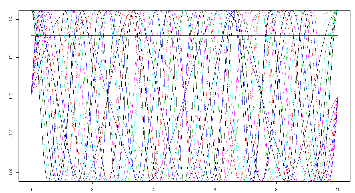
plot(mybasis)
You clearly see that:
- the maximum value is less than $\frac{1}{\sqrt \pi}$
- the Fourier basis (truncated to the first $N-2$ terms) contains a constant function (the black line), sines of increasing frequency (the curves which are equal to 0 at the domain boundaries) and cosines of increasing frequency (the curves which are equal to 1 at the domain boundaries), as it should be
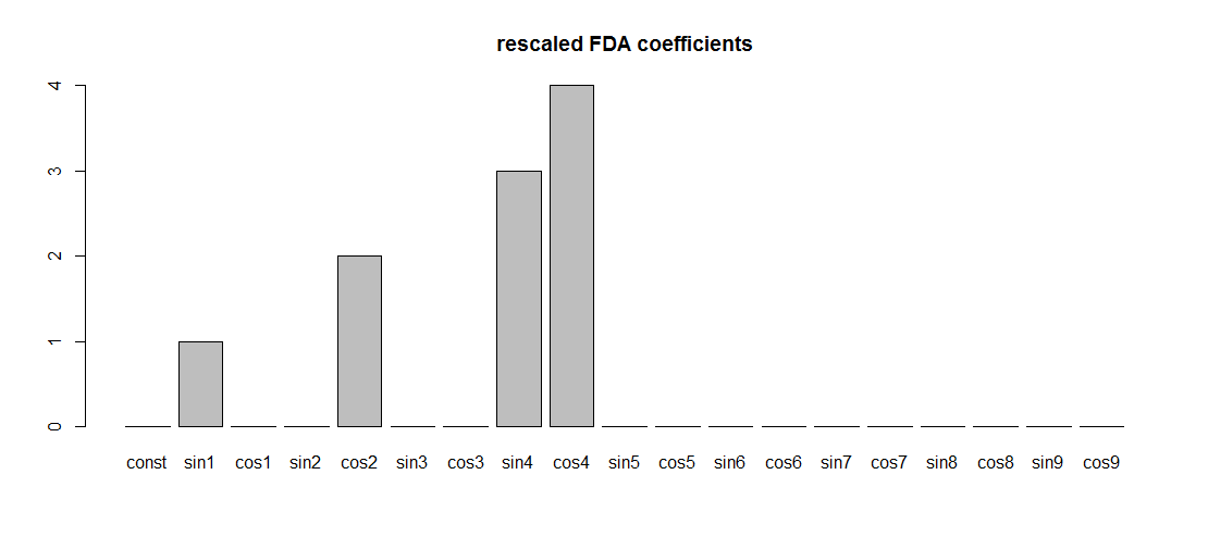
Simply scaling the Fourier basis given by fda, so that the usual Fourier basis is obtained, leads to regression coefficients having the expected values:
basisMat <- basisMat/max(abs(basisMat))
FDA_regression <- lm(Yper ~ basisMat-1)
FDA_coef <-coef(FDA_regression)
barplot(FDA_coef, names.arg = colnames(basisMat), main = "rescaled FDA coefficients")
Let's try fft now: note that since Yper is a periodic sequence, the last point doesn't really add any information (the DFT of a sequence is always periodic). Thus we can discard the last point when computing the FFT. Also, the FFT is just a fast numerical algorithm to compute the DFT, and the DFT of a sequence of real or complex numbers is complex. Thus, we really want the moduluses of the FFT coefficients:
# FFT
fft_coef <- Mod(fft(Yper[1:(N-1)]))*2/(N-1)
We multiply by $\frac{2}{N-1}$ in order to have the same scaling as with the Fourier basis ${1,\sin{ \omega x},\cos{ \omega x},\dots}$. If we didn't scale, we would still recover the correct frequencies, but the amplitudes would all be scaled by the same factor with respect to what we found before. Let's now plot the fft coefficients:
fft_coef <- fft_coef[1:((N-1)/2)]
terms <- paste0("exp",seq(0,(N-1)/2-1))
barplot(fft_coef, names.arg = terms, main = "FFT coefficients")
Ok: the frequencies are correct, but note that now the basis functions are not sines and cosines any more (they're complex exponentials $\exp{ni\omega x}$, where with $i$ I denote the imaginary unit). Note also that instead than a set of nonzero frequencies (1,2,3,4) as before, we got a set (1,2,5). The reason is that a term $x_n\exp{ni\omega x}$ in this complex coefficient expansion (thus $x_n$ is complex) corresponds to two real terms $a_n sin(n\omega x)+b_n cos(n\omega x)$ in the trigonometric basis expansion, because of the Euler formula $\exp{ix}=\cos{x}+i\sin{x}$. The modulus of the complex coefficient is equal to the sum in quadrature of the two real coefficients, i.e., $|x_n|=\sqrt{a_n^2+b_n^2}$. As a matter of fact, $5=\sqrt{3^3+4^2}$.

