Edit after @eric_kernfeld answer. I'd like to do

1. Generate a time-series, for example, from a uniform distribution.

2. Transform of non-normal variable to standard normal distribution.

3. Fit an arima model to standard normal variable.

4. Simulate from the arima model with the fitted parameters (in this case errors should be standard normal).

5. Apply the back transformation that converts simulated arima output to marginal variable.

On the steps 2 and 5 I'm going to use the Johnson transformation and the back Johnson transformation respectively.

I have a time series and I'd like to do a simulation of log-returns using the normalization with Johnson distribution.

library(JohnsonDistribution)
library(moments)

rm(list=ls(all=TRUE)) 
set.seed(1)
n <- 252
log_mydata1 <- runif(n, min=-0.06, max= 0.05)

m1   <- mean(log_mydata1)     
var1 <- sd(log_mydata1)
sk1  <- skewness(log_mydata1)
k1   <- kurtosis(log_mydata1)
# Fitting  Johnson distribution parameters and type
FitJohnsonDistribution(m1, var1, sk1, k1)
iType  <- FitJohnsonDistribution(m1, var1, sk1, k1)[1]
gamma  <- FitJohnsonDistribution(m1, var1, sk1, k1)[2]
delta  <- FitJohnsonDistribution(m1, var1, sk1, k1)[3]
lambda <- FitJohnsonDistribution(m1, var1, sk1, k1)[4]
xi     <- FitJohnsonDistribution(m1, var1, sk1, k1)[5]

# Applying Johnson transformation
z1 <- zJohnsonDistribution(log_mydata1, iType, gamma, delta, lambda , xi)
shapiro.test(z1) # W = 0.99374, p-value = 0.377

I have used the code and fitted my random data and log-returns were fitted with ARIMA(3,0,2) model. Then I applied some test to check the model quality.

# Fitting ARMA model
ArimaModelFit <- function(z)
{  
final.aic <- Inf
final.order <- c(0,0,0)
for (p in 0:3)
for (q in 0:3)
{
         if ( p == 0 && q == 0) {
             next
         }
          arimaFit = tryCatch( arima(z, order=c(p, 0, q)),
                              error=function( err ) FALSE,
                              warning=function( err ) FALSE )
         if( !is.logical( arimaFit ) ) {
             current.aic <- AIC(arimaFit)
             if (current.aic < final.aic) {
                 final.aic <- current.aic
                 final.order <- c(p, 0, q)
                 final.arima <- arima(z, order=final.order)
             }
         } else {
             next
         }
     }
result <- list(aic=final.aic, order=final.order, arima=final.arima)
return(result)
} # function

f1  <- ArimaModelFit(z1) 
rf1 <- residuals(f1$arima); shapiro.test(rf1) # W = 0.9944, p-value = 0.4785

Then I simulated data with the ARIMA model

#ARMA  Simulation
sim <- arima.sim(list(order = c(3,0,2), 
                         ar = c(f1$arima$coef[1], f1$arima$coef[2], f1$arima$coef[3]), 
                         ma = c(f1$arima$coef[4], f1$arima$coef[5])), n = n)

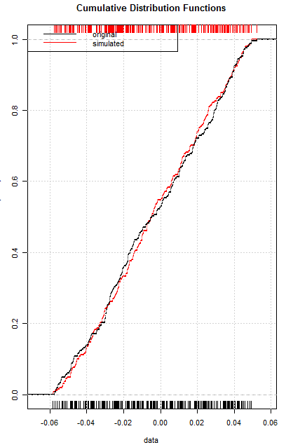
Finally, I'd like to back the fitted data to marginal variable. I have applied the Kolmogorov-Smirnov test and plotted Cumulative Distribution Functions (CDFs) of marginal (log-returns) and simulated (y) data to check the quality of 2, 3, 4, 5 step of simulation (normalization, arima, back transformation).

# Applying inverse of Johnson transformation
y <- yJohnsonDistribution(sim, iType, gamma, delta, lambda , xi)

# Two-sample Kolmogorov-Smirnov test
ks.test(log_mydata1, y) #D = 0.048552, p-value = 0.9283

    Fn = ecdf(log_mydata1)
Fm = ecdf(y)
plot(Fn,
   main="Cumulative Distribution Functions",
   xlab="data",
   ylab="Cumulative Frequency",
   pch=NA, lwd= 2,
   col = "red")
lines(Fm, pch=NA, lty=1, lwd= 2)       
rug(log_mydata1)
rug(y, side = 3, col = "red")
legend("topleft",
       legend=c("original", "simulated"),
       lty=c(1,1),
col=c("black", "red"))
grid()

The p-value of Kolmogorov-Smirnov test is 0.9283 and CDFs are close each to other.

But according to the documentaion of the JohnsonDistribution package I should use the zJohnsonDistribution function instead of the yJohnsonDistribution function.

Also I confused with sim series. In my case, sim is the normal distributed variable, but it is should be uniformly distributed on the unit interval [0, 1].

Questions. Am I correct in my steps? How to inverse correctly the Johnson normalized variable to a marginal variable? Should I use the qnorm() function?

Edit 2. I have changed the library to do the direct/back Johnson transformation:

Edit 3.

library(Johnson)
  
set.seed(1)
n <- 252
log_mydata1 <- runif(n, min=-0.06, max= 0.05)

# Applying SU Johnson transformation

jt_mydata1<-RE.Johnson(log_mydata1)
z1 <- jt_mydata1$transformed; shapiro.test(z1) # W = 0.99495, p-value = 0.5748

mean(z1); sd(z1) # -0.02276707,  1.002103

# fpar1  <- ArimaModelFit(z1)
# Coefficients:
#         ar1     ar2      ar3      ma1      ma2  intercept
#      0.5520  0.4231  -0.1234  -0.5468  -0.4532    -0.0302
# s.e.  0.3582  0.3492   0.0666   0.3572   0.3570     0.0075


#ARMA  Simulation
sim1 <- arima.sim(list(order = c(3,0,2), 
                          ar = c(0.5520,  0.4231,  -0.1234), 
                          ma = c(-0.5468,  -0.4532)), n = n)

mean(sim1);sd(sim1) #  -0.0350542, 1.041598
shapiro.test(sim1)  # W = 0.99285, p-value = 0.2675

# convert an normalized variable back to a marginal variable    
gamma1   <- jt_mydata1$f.gamma
lambda1  <- jt_mydata1$f.lambda
epsilon1 <- jt_mydata1$f.epsilon
eta1     <- jt_mydata1$f.eta
# SU
# inv_jt_mydata1 <- lambda1 * sinh((sim1 - gamma1)/eta1) +  epsilon1
# SB
inv_jt_mydata1 <- ((lambda1 + epsilon1)* exp((sim1 - gamma1)/eta1) +  epsilon1)/(1+exp((sim1 - gamma1)/eta1))

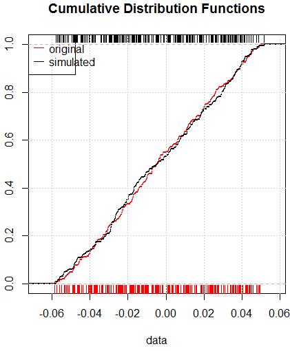
The p-value of Kolmogorov-Smirnov test is $0.97$

ks.test(log_mydata1, inv_jt_mydata1)
#    D = 0.043651, p-value = 0.97
# alternative hypothesis: two-sided

and CDFs are close each to other: