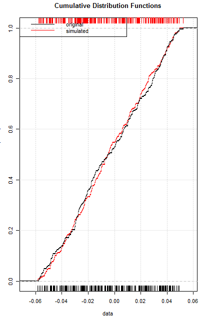
I have a time series and I'd like to do a simulation of log-returns using the normalization with Johnson distribution.

library(JohnsonDistribution)
library(moments)

rm(list=ls(all=TRUE)) 
set.seed(1)
n <- 252
log_mydata1 <- runif(n, min=-0.06, max= 0.05)

m1   <- mean(log_mydata1)     
var1 <- sd(log_mydata1)
sk1  <- skewness(log_mydata1)
k1   <- kurtosis(log_mydata1)
# Fitting  Johnson distribution parameters and type
FitJohnsonDistribution(m1, var1, sk1, k1)
iType  <- FitJohnsonDistribution(m1, var1, sk1, k1)[1]
gamma  <- FitJohnsonDistribution(m1, var1, sk1, k1)[2]
delta  <- FitJohnsonDistribution(m1, var1, sk1, k1)[3]
lambda <- FitJohnsonDistribution(m1, var1, sk1, k1)[4]
xi     <- FitJohnsonDistribution(m1, var1, sk1, k1)[5]

# Applying Johnson transformation
z1 <- zJohnsonDistribution(log_mydata1, iType, gamma, delta, lambda , xi)
shapiro.test(z1) # W = 0.99374, p-value = 0.377

I have used the code and fitted my random data and log-returns were fitted with ARIMA(3,0,2) model. Then I applied some test to check the model quality.

# Fitting ARMA model
ArimaModelFit <- function(z)
{  
final.aic <- Inf
final.order <- c(0,0,0)
for (p in 0:3)
for (q in 0:3)
{
         if ( p == 0 && q == 0) {
             next
         }
          arimaFit = tryCatch( arima(z, order=c(p, 0, q)),
                              error=function( err ) FALSE,
                              warning=function( err ) FALSE )
         if( !is.logical( arimaFit ) ) {
             current.aic <- AIC(arimaFit)
             if (current.aic < final.aic) {
                 final.aic <- current.aic
                 final.order <- c(p, 0, q)
                 final.arima <- arima(z, order=final.order)
             }
         } else {
             next
         }
     }
result <- list(aic=final.aic, order=final.order, arima=final.arima)
return(result)
} # function

f1  <- ArimaModelFit(z1) 
rf1 <- residuals(f1$arima); shapiro.test(rf1) # W = 0.9944, p-value = 0.4785

Then I simulated data with the ARIMA model

#ARMA  Simulation
sim <- arima.sim(list(order = c(3,0,2), 
                         ar = c(f1$arima$coef[1], f1$arima$coef[2], f1$arima$coef[3]), 
                         ma = c(f1$arima$coef[4], f1$arima$coef[5])), n = n)

Finally, I'd like to inverse the fitted data and to chect the quality of simulation with Kolmogorov-Smirnov test and Cumulative Distribution Functions (CDFs) of marginal (log-returns) and simulated (y) data.

# Applying inverse of Johnson transformation
y <- yJohnsonDistribution(sim, iType, gamma, delta, lambda , xi)

# Two-sample Kolmogorov-Smirnov test
ks.test(log_mydata1, y) #D = 0.048552, p-value = 0.9283

    Fn = ecdf(log_mydata1)
Fm = ecdf(y)
plot(Fn,
   main="Cumulative Distribution Functions",
   xlab="data",
   ylab="Cumulative Frequency",
   pch=NA, lwd= 2,
   col = "red")
lines(Fm, pch=NA, lty=1, lwd= 2)       
rug(log_mydata1)
rug(y, side = 3, col = "red")
legend("topleft",
       legend=c("original", "simulated"),
       lty=c(1,1),
col=c("black", "red"))
grid()

The p-value of Kolmogorov-Smirnov test is 0.9283 and CDFs are close each to other.

But according to the documentaion of the JohnsonDistribution package I should use the zJohnsonDistribution function instead of the yJohnsonDistribution function.

Also I confused with sim series. In my case, sim is the normal distributed variable, but it is should be uniformly distributed on the unit interval [0, 1].

Questions. Am I correct in my steps? How to inverse correctly the Johnson normalized variable to a marginal variable? Should I use the qnorm() function?