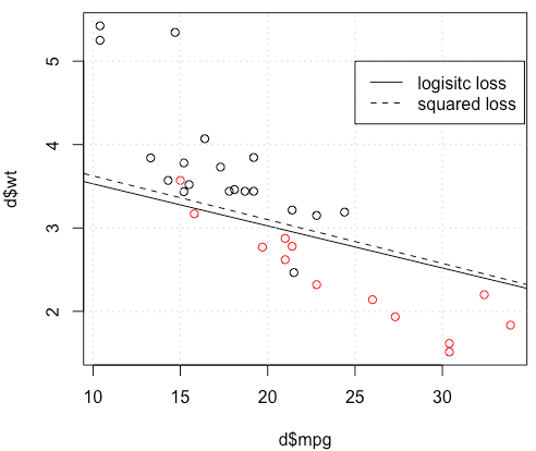
I am trying to use squared loss to do binary classification. The loss is $\sum_i (y_i-p_i)^2$ where $y_i$ is the ground truth label (0 or 1) and $p_i$ is the predicted probability $p_i=\text{Logit}^{-1}(\beta^Tx_i)$.

In other words, I am replace logistic loss with squared loss in classification setting, other parts are the same.

For a toy example with mtcars data, in many cases, I got a model "similar" to logistic regression (see following figure, with random seed 0).

But in somethings (if we do set.seed(1)), squared loss seems not working well.

What is happening here? The optimization does not converge? Logistic loss is easier to optimize comparing to squared loss? Any help would be appreciated.

Code

d=mtcars[,c("am","mpg","wt")]
plot(d$mpg,d$wt,col=factor(d$am))
lg_fit=glm(am~.,d, family = binomial())
abline(-lg_fit$coefficients[1]/lg_fit$coefficients[3],
       -lg_fit$coefficients[2]/lg_fit$coefficients[3])
grid()

# sq loss
lossSqOnBinary<-function(x,y,w){
  p=plogis(x %*% w)
  return(sum((y-p)^2))
}

# ----------------------------------------------------------------
# note, this random seed is important for squared loss work
# ----------------------------------------------------------------
set.seed(0)

x0=runif(3)
x=as.matrix(cbind(1,d[,2:3]))
y=d$am
opt=optim(x0, lossSqOnBinary, method="BFGS", x=x,y=y)

abline(-opt$par[1]/opt$par[3],
       -opt$par[2]/opt$par[3], lty=2)
legend(25,5,c("logisitc loss","squared loss"), lty=c(1,2))