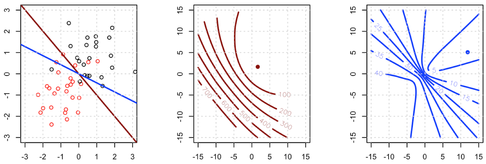
As @Chaconne mentioned, the problem is squared loss for classification is non-convex and harder to optimize. To add on @Chaconne's math, I would like to present some visualizations on to different objective functions.
We will change the demo data from mtcars, since the original toy example has $3$ coefficients including the intercept. We will use another toy data set generated from mlbench, in this data set, we set $2$ parameters, so it is possible to make better visualization.
The data is shown in the left figure: we have two classes. The middle figure and right figure shows the contour for logistic loss (red) and squared loss (blue).
From the contour we can easily see how why optimizing squared loss is harder: as Chaconne mentioned, it is non-convex.
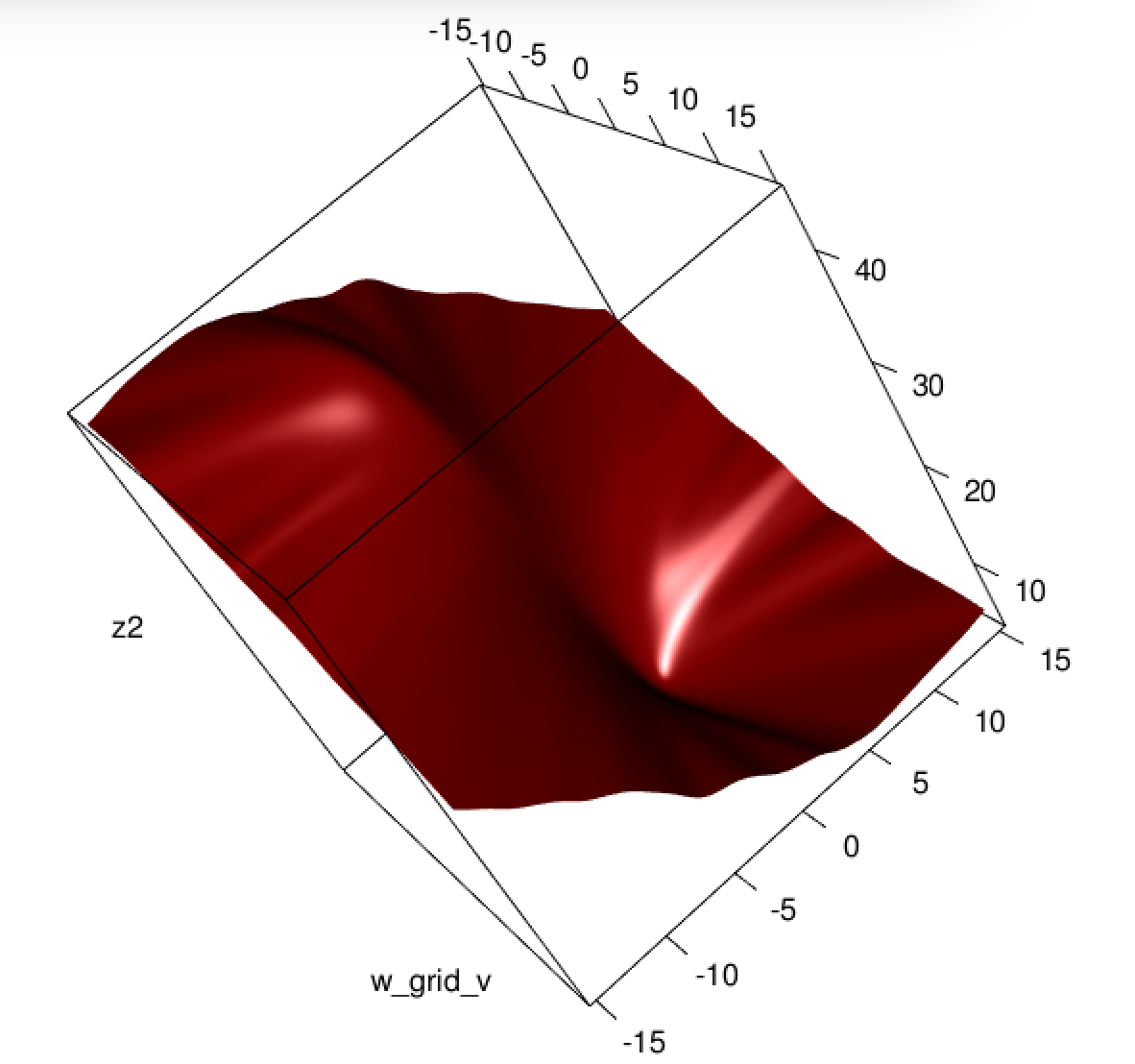
Here is one more view from persp3d.
Code
set.seed(0)
d=mlbench::mlbench.2dnormals(50,2,r=1)
x=d$x
y=ifelse(d$classes==1,1,0)

lg_loss <- function(w){
  p=plogis(x %*% w)
  L=-y*log(p)-(1-y)*log(1-p)
  return(sum(L))
}
sq_loss <- function(w){
  p=plogis(x %*% w)
  L=sum((y-p)^2)
  return(L)
}

w_grid_v=seq(-15,15,0.1)
w_grid=expand.grid(w_grid_v,w_grid_v)

opt1=optimx::optimx(c(1,1),fn=lg_loss ,method="BFGS")
z1=matrix(apply(w_grid,1,lg_loss),ncol=length(w_grid_v))

opt2=optimx::optimx(c(1,1),fn=sq_loss ,method="BFGS")
z2=matrix(apply(w_grid,1,sq_loss),ncol=length(w_grid_v))

par(mfrow=c(1,3))
plot(d,xlim=c(-3,3),ylim=c(-3,3))
abline(0,-opt1$p2/opt1$p1,col='darkred',lwd=2)
abline(0,-opt2$p2/opt2$p1,col='blue',lwd=2)
grid()
contour(w_grid_v,w_grid_v,z1,col='darkred',lwd=2, nlevels = 8)
points(opt1$p1,opt1$p2,col='darkred',pch=19)
grid()
contour(w_grid_v,w_grid_v,z2,col='blue',lwd=2, nlevels = 8)
points(opt2$p1,opt2$p2,col='blue',pch=19)
grid()


# library(rgl)
# persp3d(w_grid_v,w_grid_v,z1,col='darkred')


