Dan and Michael point out the relevant issues. Just for completeness, the relationship between adjusted $R^2$ and $R^2$ is given by (see, e.g., here)
$$ R^2_{adjusted}=1-(1-R^2)\frac{n-1}{n-K}, $$ (with $K$ the number of regressors, including the constant). This shows that $R^2_{adjusted}=1$ if $R^2=1$, unless (see below) $K=n$.
$R^2=1$ occurs when all residuals $\hat u_i=y_i-\hat y_i$ are zero, as $$ R^2=1-\frac{\hat{u}'\hat{u}/n}{\tilde{y}'\tilde{y}/n}. $$ Here, $\hat u$ denotes the vector of residuals and $\tilde y$ the vector of demeaned observations on the dependent variable.
Dan discusses one reason to get an $R^2$ of 1. Another is to have as many regressors as observations, i.e., $K=n$.
Technically, this is because the $n\times K$ regressor matrix $X$ then is square. The OLS estimator $\hat\beta=(X'X)^{-1}X'y$ can then be written as (assuming no exact multicollinearity) $$ \hat\beta=(X'X)^{-1}X'y=X^{-1}{X'}^{-1}X'y=X^{-1}y $$ so that the fitted values $\hat y=X\hat\beta$ are just $\hat y=XX^{-1}y=y$, so that all residuals are zero.
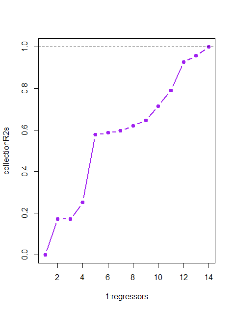
Here is an illustration using artificial data (code below), in which regressors are generated totally independently of $y$, and yet we achieve an $R^2$ of 1 once we have as many of them as we have observations.

Code:
n <- 15
regressors <- n-1 # enough, as we'll also fit a constant
y <- rnorm(n)
X <- matrix(rnorm(regressors*n),ncol=regressors)

collectionR2s <- rep(NA,regressors)
for (i in 1:regressors){
  collectionR2s[i] <- summary(lm(y~X[,1:i]))$r.squared
}
plot(1:regressors,collectionR2s,col="purple",pch=19,type="b",lwd=2)
abline(h=1, lty=2)
When $K=n$, R however, correctly, does not report an adjusted $R^2$:
> summary(lm(y~X))

Call:
lm(formula = y ~ X)

Residuals:
ALL 15 residuals are 0: no residual degrees of freedom!

Coefficients:
            Estimate Std. Error t value Pr(>|t|)
(Intercept)  2.36296         NA      NA       NA
X1          -1.09003         NA      NA       NA
X2           0.39177         NA      NA       NA
X3           0.19273         NA      NA       NA
X4           0.51528         NA      NA       NA
X5          -0.04530         NA      NA       NA
X6          -1.28539         NA      NA       NA
X7          -0.72770         NA      NA       NA
X8          -0.14604         NA      NA       NA
X9           0.34385         NA      NA       NA
X10         -0.93811         NA      NA       NA
X11          2.23064         NA      NA       NA
X12          0.06744         NA      NA       NA
X13          0.21220         NA      NA       NA
X14         -2.29134         NA      NA       NA

Residual standard error: NaN on 0 degrees of freedom
Multiple R-squared:      1, Adjusted R-squared:    NaN
F-statistic:   NaN on 14 and 0 DF,  p-value: NA
