The outlier rule is based on the inter-quartile range (upper minus lower quartile).
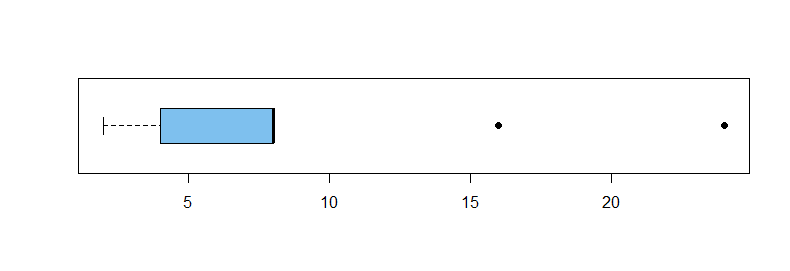
Your data. If you have so many RAM values at 4 and 8 that those are the lower and upper quartiles, respectively, then $\text{IQR} = 8 - 4 = 4,$ and any value above $Q_3 + 1.5(\text{IQR}) = 8 + 1.5(4) = 14$ will show as a high outlier. A small-sample version follows:
x = c(2,2,4,4,4,4,4,4,8,8,8,8,8,8,8,8,16,16,16,24,24)
summary(x)
   Min. 1st Qu.  Median    Mean 3rd Qu.    Max.
  2.000   4.000   8.000   8.952   8.000  24.000
IQR(x)
[1] 4

boxplot(x, horizontal=T, col="skyblue2", pch=19)
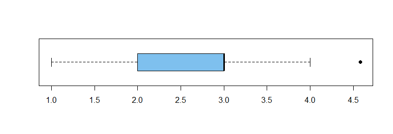
If you take logs of your observations, a boxplot may be somewhat better suited as a graphical description.
y = log2(x)
summary(y)
   Min. 1st Qu.  Median    Mean 3rd Qu.    Max.
  1.000   2.000   3.000   2.818   3.000   4.585
IQR(y)
[1] 1
boxplot(y, horizontal=T, col="skyblue2", pch=19)
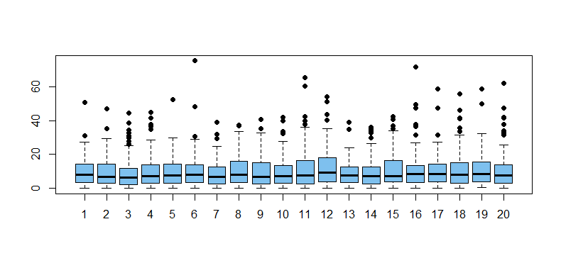
Outliers are common in exponential data. It is a characteristic of samples from right-skewed distributions to show numerous 'outliers'. Below are boxplots for 20 samples of size $n = 100$ from an exponential distribution with mean 10.
m = 20;  n = 100;  x = rexp(m*n, .1);  g = rep(1:20, each=100)
boxplot(x ~ g, col="skyblue2", pch=19)
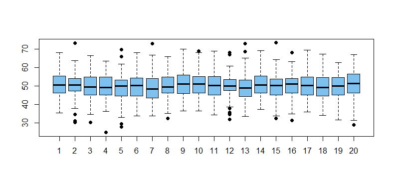
Outliers are not rare in normal data. Moreover, slightly more than half of normal samples of size $n = 100$ show at least one outlier.
set.seed(606)
nr.out = replicate(10^5,
          length(boxplot.stats(rnorm(100, 50, 7))$out))
mean(nr.out >= 1)
[1] 0.52505
    nr.out
      0       1       2       3       4       5       6       7
0.47495 0.28644 0.13589 0.06059 0.02475 0.01010 0.00439 0.00171
      8       9      10      11      12      13
0.00073 0.00027 0.00007 0.00006 0.00004 0.00001
Boxplots for 20 of the 100,000 normal samples from the simulation above are shown below.
Note: Applied to a normal population the outlier rule would label observations more than about 2.7 SDs from the mean as outliers. Samples do not precisely emulate populations, but normal tails have enough probability that it is not rare for moderately large samples to have some outliers. Boxplot 'outliers' are worth a second look, but they are by no means necessarily 'errors'.
qnorm(.75) + 1.5*diff(qnorm(c(.25,.75)))
[1] 2.697959
2*pnorm(-2.7)
[1] 0.006933948


