Comment on lognormal and normal distributions.
The variance of data tends to decrease when you take logs of the values. Perhaps the most common case is that, if $X_1$ is lognormal, then $X_2 = \ln(X_1)$ is normal, which has smaller variance than $X_1.$ Also, $X_3 = \ln(X_2)$ has a still smaller variance.
Below we begin with a random sample (using R) of $n = 10^4$ observations from a lognormal distribution with parameters $\mu = 50, \sigma = 2.$ (It is customary to use lognormal parameters that match parameters of the related normal distribution. You can look at Wikipedia on 'lognormal distributions' for details.) We show means and standard deviations for distributions of $X_1, X_2,$ and $X_3.$
set.seed(720); n = 10^4
x2 = rnorm(n, 50, 2);  x1 = exp(x2);  x3 = log(x2)
mean(x1); mean(x2); mean(x3)
[1] 3.686093e+22
[1] 50.01289         # aprx E(X2) = 50
[1] 3.911481
sd(x1); sd(x2); sd(x3)
[1] 2.308712e+23
[1] 1.997261         # aprx SD(X2) = 2
[1] 0.04004551
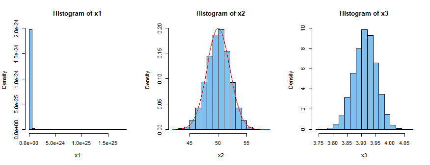
Then we show histograms of the three samples. At the left, notice that it is difficult to make an informative histogram of $X_1$ because it is so severely skewed to the right. In the center panel, we overlay the density function of $\mathsf{Norm}(\mu =50, \sigma=2);$ which is symmetrical. At the right, notice that taking (natural) logs once again results in a slightly left-skewed distribution.
Notes: (1) The the support of a lognormal distribution is $(0, \infty).$ A normal distribution may take negative values.
(2) R code for the figure:
par(mfrow=c(1,3))
hist(x1, prob=T, br=50, col="skyblue2")
hist(x2, prob=T, col="skyblue2")
  curve(dnorm(x,50,2), add=T, col="red")
hist(x3, prob=T, col="skyblue2")
par(mfrow=c(1,1))

