Difference 1
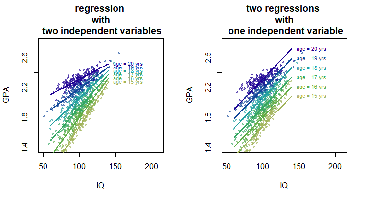
Below is a sketch of a hypothetical relationship for GPA as function of age and IQ. Added to this are the fitted lines for the two different situations.
If you add the effects of two regressions with one independent variable then you can see this as obtaining a relationship for the slope of GPA as function of IQ and the slope of GPA as function of age. Together this relates to the curves of the one relation shifting up or down as function of the other independent parameter.
However, when you do a regression with the two independent variables at once then the model also takes into account a variation of the slope as a function of both age and IQ.
For instance in the hypothetical case below the increase of GPA as function of increase in IQ is not the same for each age and the effect of IQ is stronger at lower age than at higher age.
layout(matrix(1:2,1))

# sample of 1k people with different ages and IQ
IQ <- rnorm(10^3,100,15)
age <- sample(15:20,10^3,replace=TRUE)

# hypothetical model for GPA
set.seed(1)
GPA_offset <- 2
IQ_slope <- 1/100
age_slope <- 1/8
interaction <- -1/500
noise <- rnorm(10^3,0,0.05)

GPA <- GPA_offset +
       IQ_slope * (IQ-100) +
       age_slope * (age - 17.5) +
       interaction * (IQ-100) * (age - 17.5) +
       noise

# plotting with fitted models


cols <- hsv(0.2+c(0:5)/10,0.5+c(0:5)/10,0.7-c(0:5)/40,0.5)
cols2 <- hsv(0.2+c(0:5)/10,0.5+c(0:5)/10,0.7-c(0:5)/40,1)
plot(IQ,GPA,
     col = cols[age-14], bg = cols[age-14], pch = 21, cex=0.5,
     xlim = c(50,210), ylim = c(1.4,2.8))

mod <- lm(GPA ~ IQ*age)

for (i in c(15:20)) {
  xIQ <- c(60,140)
  yGPA <- coef(mod)[1] + coef(mod)[3] * i + (coef(mod)[2] + coef(mod)[4] * i) * xIQ
  lines(xIQ, yGPA,col=cols2[i-14],lwd = 2)
  text(xIQ[2], yGPA[2], paste0("age = ", i, " yrs"), pos=4, col=cols2[i-14],cex=0.7)
}
title("regression \n with \n two independent variables")


cols <- hsv(0.2+c(0:5)/10,0.5+c(0:5)/10,0.7-c(0:5)/40,0.5)
plot(IQ,GPA,
     col = cols[age-14], bg = cols[age-14], pch = 21, cex=0.5,
     xlim = c(50,210), ylim = c(1.4,2.8))

mod <- lm(GPA ~ IQ+age)

for (i in c(15:20)) {
  xIQ <- c(60,140)
  yGPA <- coef(mod)[1] + coef(mod)[3] * i + (coef(mod)[2] ) * xIQ
  lines(xIQ, yGPA,col=cols2[i-14],lwd = 2)
  text(xIQ[2], yGPA[2], paste0("age = ", i, " yrs"), pos=4, col=cols2[i-14],cex=0.7)
}

title("two regressions \n with \n one independent variable")
Difference 2
What if IQ and age are slightly correlated in practice?
The above explains the difference based on the consideration of the additional interaction term. But even without the interaction term one might obtain different results between the single and multiple regressions.
This occurs when the experimental design is not balanced and the independent variables correlate. E.g. consider Simpson's paradox.

