Return to Revisions

I can imagine a frequentist density forecast/prediction as something like a distribution of intervals.

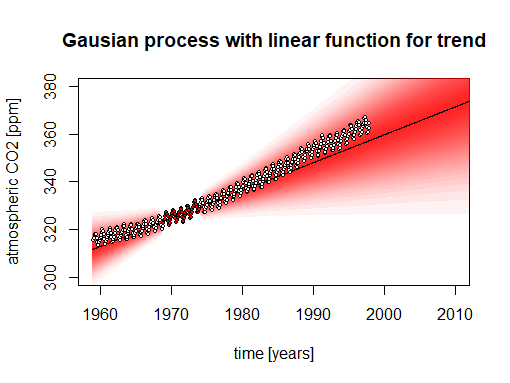
For instance providing something like the image below which is an image containing multiple confidence boundary lines (the original is here with only a single 95% confidence interval). And something similar can be done with prediction intervals.

With this interpretation the difference between the frequentist density and the Bayesian density corresponds to the difference between a confidence interval and a credible interval. Those two are not the same.

We could say that:

1. The Bayesian analysis uses more/different information (it includes a posterior distribution for the distribution of parameters, either based on former knowledge or based on assumptions/believes)
2. The Bayesian analysis expresses a probability in a different way.

• The confidence interval relates to 'the probability of the observation given the parameters'.
• The credible interval relates to the 'probability of the parameters given the observation'.

Contrast between confidence interval and prediction interval

The intuition above relies a lot on confidence intervals, but similar things can be said about prediction intervals.

The confidence intervals are maybe more easy to interpret than prediction intervals. Prediction intervals include the error of the mean (which can be seen to coincide with confidence intervals) plus an estimate of the random noise.

It is more difficult to give prediction intervals a same frequentist interpretation, although an alternative way to look at is that for frequentist prediction intervals you can say that 'the frequentist prediction interval will contain the future observation a fraction $x \%$ of the time'.

So the difference between frequentist prediction intervals and Bayesian prediction intervals is still that the Bayesian intervals use more information, but the frequentist prediction interval are independent of from the parameter distribution and 'work' independent from the prior distribution (given that the model is correct).

I imagine that the following interpretation still works 'the frequentist prediction interval relates to the probability of the observation given the predicted value, it is the collection of those predicted values for which the prior observed effects/data/statistics occurs within a region with $x \%$ probability'.

Example prediction of a value for a Gaussian distribution population

When creating a confidence interval for the estimate of the mean of Gaussian distributed population then one can use a t-distribution and this has a geometrical interpretation. The same geometrical interpretation will work for the estimate of a prediction interval.

Let $X_i \sim N(\mu, \sigma)$ and say we observe a sample $X_1, ... , X_n$ of size $n$ and wish to predict $X_{n+1}$.

We can construct a frequentist prediction interval with the interpretation that

• No matter what the value of $\mu$ and $\sigma$ is, the value $X_{n+1}$ will be $x\%$ of the time inside the prediction interval.

but also:

• Given a hypothetical predicted value $\tilde{X}_{n+1}$ in the prediction range, the observations $\bar{X}$ and $s$ (the sample mean and sample deviation) will be occuring within some range that occurs $x$ percent of the time. (That means we will only include those values in the prediction range for which we make our observations $x\%$ of the time, such that we will never fail more than $x\%$ of the time)

So instead of considering the distribution of $X_{n+1}$ given the data $\bar{X}$ and $s$, we consider the other way around, we consider the distribution of the data $\bar{X}$ and $s$ given $X_{n+1}$.

(we can plot this distribution because $\bar{X}-X_{n+1}$ is Gaussian distributed, and $s$ has a scaled chi-distribution)

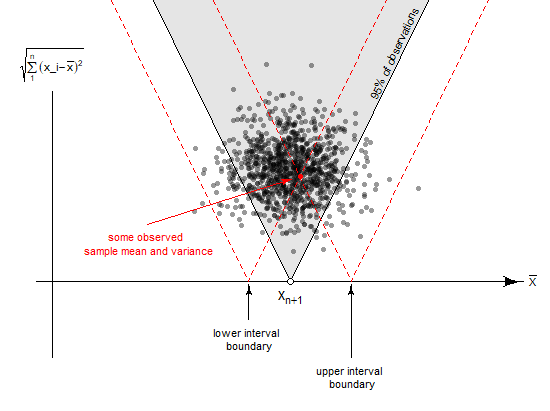
• In the image above you see the distribution of the sample standard deviation and the sample mean given a value for $X_{n+1}$.

The distribution of this deviation can be bounded by a cone (in the image 95%) and this is independent of $\sigma$ (because both variables, normal distributed and scaled chi distributed) scale the same when $\sigma$ changes thus the distribution of the angle does not change.

• And the red dotted lines show how you can construct the prediction interval. For a given observation (the red dot), when you have a variable within this range the observation will be inside the 'cone of 95%' for those predicted values.

Thus this prediction interval has an interpretation like a confidence interval: It relates to the probability of the data, given the predicted value (instead of the inverse 'the probability of the predicted value, given the data').

Code for the image:

# settings
set.seed(1)
n <- 10^3
smp = 10

# hypothetical x[n+1]
xn1 <- 7.5

# simulate data and compute statistics
X <- matrix(rnorm(smp*n),n)
prd <- rnorm(n)          
diff <- rowMeans(X)-prd
rss <- sqrt(rowSums((X-rowMeans(X))^2))

#plotting
dev.off()
par(mar=c(0,0,0,0))

plot(xn1+diff, rss, bty = 'n', ylim = c(-3,7), xlim = c(-1,15), xaxt = "n", yaxt = "n", xlab="", ylab = "",
     pch=21,col=rgb(0,0,0,0),bg=rgb(0,0,0,0.4),cex=0.7)

Arrows(-0.5,0,14.5,0,arr.length=0.4)
lines(c(0,0),c(-2,5))

text(0,5,expression(sqrt(sum((x_i-bar(x))^2,i=1,n))),pos=3,cex=0.7)
text(14.7,0,expression(bar(X)),pos=4,cex=0.7)


qt(0.95,smp-1)

ang <- sqrt((smp-1)*(1+1/smp))/qt(0.95,smp-1)

lines(c(xn1-10,xn1,xn1+10),c(10,0,10)*ang)
polygon(c(xn1-10,xn1,xn1+10),c(10,0,10)*ang, 
        col = rgb(0,0,0,0.1), border = NA, lwd=0.01)

text(10.7,6,"95% of observations",srt=65,cex=0.7)

points(xn1, 0, pch=21, col=1, bg = "white")     
text(xn1,0,expression(x[n+1]),pos=1)

points(xn1+diff[1],rss[1],pch=21,col=2,bg=2,cex=0.7)


lines(diff[1]+rss[1]/ang+c(xn1-10,xn1,xn1+10),c(10,0,10)*sqrt((smp-1)*(1+1/smp))/qt(0.95,smp-1),col=2,lty=2)
lines(diff[1]-rss[1]/ang+c(xn1-10,xn1,xn1+10),c(10,0,10)*sqrt((smp-1)*(1+1/smp))/qt(0.95,smp-1),col=2,lty=2)


Arrows(xn1+diff[1]+rss[1]/ang,-2,xn1+diff[1]+rss[1]/ang,-0.2,col=1,cex=0.5,arr.length=0.2)
Arrows(xn1+diff[1]-rss[1]/ang,-1,xn1+diff[1]-rss[1]/ang,-0.2,col=1,cex=0.5,arr.length=0.2)

text(xn1+diff[1]-rss[1]/ang,-1.0,"lower interval \n boundary",pos=1,srt=0,cex=0.7)
text(xn1+diff[1]+rss[1]/ang,-2.0,"upper interval \n boundary",pos=1,srt=0,cex=0.7)



Arrows(3,1.5,xn1+diff[1]-0.4,rss[1]-0.1,col=2,cex=0.5,arr.length=0.2)
text(3,1.5,"some observed \n sample mean and variance",col=2,pos=1,srt=0,cex=0.7)