I can suggest three other methods which can be better in some sense than adding noise.

shuffling noise around

Instead of adding noise, let's push it around! We'll shuffle noise between two variables so that the correlation is what we want while preserving variances of each variable. Here's the final result for S&P 500 and Apple returns in 2020 Jan-Apr, where original correlation was 94% which I changed into -70%:

I used PCA and Cholesky decomposition to do this:

• apply PCA to destandardized original series X to get the uncorrelated series F
• standardize PC factors F to get unit variance series U
• apply Cholesky decomposition to standardized uncorrelated series U to obtain correlated series Y with unit variance
• destandardize Y to get to the series with original means and variances X'

This looks a bit intimidating, but you don't have to do this manually, and can use software. We don't introduce external noise. We only push the noise that exists in the data already from one place to another. Total variance of the data set remains the same as well as some other characteristics such as means.

re-ordering variables

Second method is to not change the observations at all, but instead rearrange the observations in variables in such a way that correlation changes. Consider this: if I take random samples from both series, and calculate the correlation between these samples, then correlation will be zero. So, simple rearranging the order in variables will change correlation.

Advantage of this method is that variances remain the same, and overall distributions remain intact in the dataset. Since, you work with stock return, there's no autocorrelation, so rearranging doesn't impact this aspect at all, at least in theory

Rotation and scale

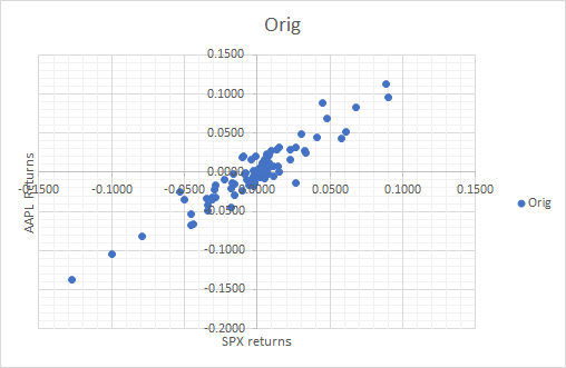
I can transform one of the variables in such a way that the other stays the same but correlation changes. It's a simple rotation and scale with a possible flip. Look at the scatter plot of the original series:

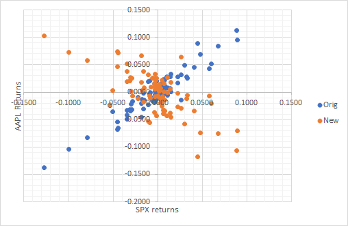
Now, imagine that I flip the Y axis and scale it so that new series will have different correlation but X-axis values remain the same, i.e. S&P 500 returns are preserved. This is how you do it.

Get new series Y as from original series X by solving for a and b: $$y_1=x_1\\ y_2=ax_1+bx_2\\var[y_2]=var[x_2]=\sigma_2^2\\cov[x_1,x_2]=\rho\sigma_1\sigma_2\\cov[y_1,y_2]=c\sigma_1\sigma_2$$

Write down variance and covariance of $y_2$: $$var[y_2]=a^2\sigma_1^2+b^2\sigma_2^2+2ab\rho\sigma_1\sigma_2\equiv\sigma_2^2$$ $$cov[y_1,y_2]=a\sigma_1^2+b\rho\sigma_1\sigma_2=c\sigma_1\sigma_2$$

You have two nonlinear equations and two unknowns a,b. You can solve this analytically or like me, a lazy guy, numerically with Excel solver, which got me:

• a = 1.375
• b = -2.0213

and the following plot of new series, where you can see that SPX returns remained the same and only AAPL returns changed while mean and variance were preserved: