First, since OP's problem is with relation to stock and index returns correlation, I must note that one thing to be aware of is that if the stock, such as AAPL, is a part of index such as SPX, then the problem is a little more complex, because any change to AAPL will spill into SPX index.

So, let's assume that the stock in question is not a constituent of SPX index. In this case I offer you two and half methods. First two would preserve the index as is, and the last one will not, but it will not add external noise either.

mix-in noises with one variable staying the same

I can transform one of the variables in such a way that the other stays the same but correlation changes. It's a simple mixing in the noise from first variable into the second. This is how you do it.

Get new series Y as from original series X by solving for a and b: $$y_1=x_1\\ y_2=ax_1+bx_2\\var[y_2]=var[x_2]=\sigma_2^2\\cov[x_1,x_2]=\rho\sigma_1\sigma_2\\cov[y_1,y_2]=c\sigma_1\sigma_2$$

Write down variance and covariance of $y_2$: $$var[y_2]=a^2\sigma_1^2+b^2\sigma_2^2+2ab\rho\sigma_1\sigma_2\equiv\sigma_2^2$$ $$cov[y_1,y_2]=a\sigma_1^2+b\rho\sigma_1\sigma_2=c\sigma_1\sigma_2$$ $$a\sigma_1+b\rho\sigma_2=c\sigma_2$$

You have two nonlinear equations and two unknowns a,b. You can solve this analytically or like me, a lazy guy, numerically with Excel solver, which got me:

• a = 1.375
• b = -2.0213

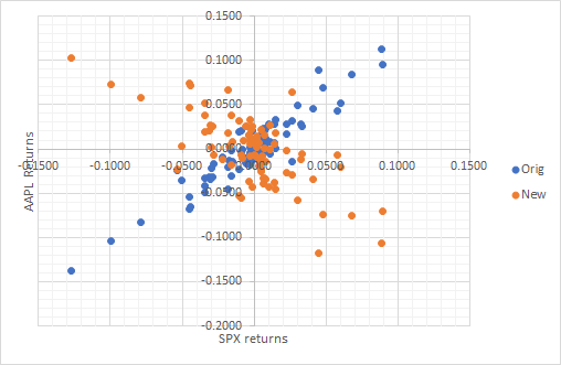
and the following plot of new series, where you can see that SPX returns remained the same and only AAPL returns changed while mean and variance were preserved:

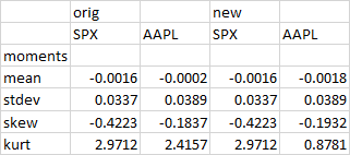
Here's the first four moments after the transformation:

Note, that only kurtosis has changed significantly, yet it's a very important moment in portfolio management, for it is responsible for a lot of tail risk. In this case, the tail of the second variable thinnedconsiderably.

re-ordering variables

Second method is to not change the observations at all, but instead rearrange the observations in variables in such a way that correlation changes. Consider this: if I take random samples from both series, and calculate the correlation between these samples, then correlation will be zero. So, simple rearranging the order in variables will change correlation.

Advantage of this method is that variances remain the same, and overall distributions remain intact in the dataset. Since, you work with stock return, there's no autocorrelation, so rearranging doesn't impact this aspect at all, at least in theory. I don't know whether this method can generate drastic changes in correlation such flipping its sign like in the example above.

shuffling noise around

Instead of adding noise, let's push it around! We'll shuffle noise between two variables so that the correlation is what we want while preserving variances of each variable. Here's the final result for S&P 500 and Apple returns in 2020 Jan-Apr, where original correlation was 94% which I changed into -70%:

I used PCA and Cholesky decomposition to do this:

• apply PCA to destandardized original series X to get the uncorrelated series F
• standardize PC factors F to get unit variance series U
• apply Cholesky decomposition to standardized uncorrelated series U to obtain correlated series Y with unit variance
• destandardize Y to get to the series with original means and variances X'

This looks a bit intimidating, but you don't have to do this manually, and can use software. We don't introduce external noise. We only push the noise that exists in the data already from one place to another. Total variance of the data set remains the same as well as some other characteristics such as means.

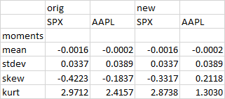
Here's the first 4 moments after the transformation:

You can see how the higher moments change, especially, kurtosis. If the stock returns were normal, then this wouldn't have happened. However, the stock return usually have heavier tails than normal. So, watch out for thinner tails if you are analyzing tail risk metrics.