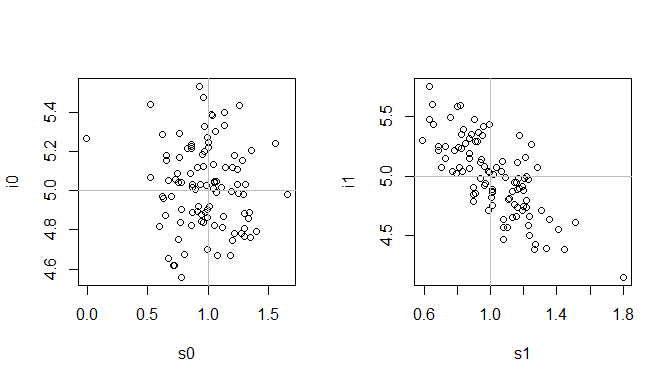
There is a sense in which it is 'bad' for covariates to be highly correlated in a regression model, namely, that it can lead to multicollinearity. However, I don't think it's very meaningful to claim that correlation between the slope and the intercept to be correlated.
That said, your question is really about how there can be a correlation between the slope and the intercept, when these are always just $2$ points. This confusion is perfectly sensible. The problem is that the fact has been stated in an imprecise way. (I'm not being critical of whomever wrote that—I speak like that all the time.)
A more precise way to state the underlying fact is that the sampling distributions of the slope and intercept are correlated. An easy way to see this is through a simple simulation: Generate (pseudo)random samples of $X$ and $Y$ data from a single data generating process, fit a simple regression model in the same way to each sample, and store the estimates. Then you can compute the correlation, or plot them as you like.
set.seed(6781)  # this makes the example exactly reproducible

B         = 100  # the number of simulations we'll do
N         =  20  # the number of data in each sample
estimates = matrix(NA, nrow=B, ncol=4)  # this will hold the results
colnames(estimates) = c("i0", "s0", "i1", "s1")
for(i in 1:B){
  x0 = rnorm(N, mean=0, sd=1)  # generating X data w/ mean 0
  x1 = rnorm(N, mean=1, sd=1)  # generating X data w/ mean 1
  e  = rnorm(N, mean=0, sd=1)  # error data
  y0 = 5 + 1*x0 + e            # the true data generating process
  y1 = 5 + 1*x1 + e
  m0 = lm(y0~x0)               # fitting the models
  m1 = lm(y1~x1)
  estimates[i,1:2] = coef(m0)  # storing the estimates
  estimates[i,3:4] = coef(m1)
}
cor(estimates[,"i0"], estimates[,"s0"])  # [1] -0.06876971  # uncorrelated
cor(estimates[,"i1"], estimates[,"s1"])  # [1] -0.7426974   # highly correlated
windows(height=4, width=7)
  layout(matrix(1:2, nrow=1))
  plot(i0~s0, estimates)
  abline(h=5, col="gray")  # these are the population parameters
  abline(v=1, col="gray")
  plot(i1~s1, estimates)
  abline(h=5, col="gray")
  abline(v=1, col="gray")
For some related information, it may help to read some of my other answers:
- How to interpret coefficient standard errors in linear regression?
- Are all slope coefficients correlated with the intercept in multiple linear regression?
- Why does the standard error of the intercept increase the further x¯ is from 0?
Edit:
From your comments, I gather your concern is based on the following quote:
in complex models, strong correlations like this can make it difficult to fit the model to the data. So we’ll want to use some golem engineering tricks to avoid it, when possible. The first trick is centering.
From:
- McElreath, R. (2015). Statistical Rethinking: A Bayesian Course with Examples in R and Stan. Chapman & Hall.
(Note that I haven't read the book.) The author's concern is perfectly reasonable, but it doesn't really have anything to do with the quality of the model or the inferences that it will support. The issue is with computational problems that could arise in the methods used to estimate the model. Note further that centering does not change anything substantive about the model, and that this is an issue in Bayesian estimation, but won't be a problem for frequentist models (like those above) that are estimated via ordinary least squares.
It may help to read:

