I'm struggling with the interpretation of orthogonal polynomial interactions when both predictors are continuous and would like to make sure my interpretation is correct. Thank you in advance for your help.

Summary of the Design

42 subjects produced two items, which were evaluated by 80 raters. The outcome variable in our analysis is binary (0/1), and we have three continuous predictors and a number of covariates. We are interested in evaluating two hypotheses:

1. A and B predict D.
2. The relationship between A/B and D depends on C.

Testing the first hypothesis is straightforward, but the second one is causing us some trouble because we are interested in evaluating the linear and quadratic moderating effect of C on the relationship between A/B and D. We standardized all continuous predictors and created orthogonal polynomials using the polypoly function. We opted to use the polypoly instead of poly to add the orthogonal polynomials to the data frame and to bring the scale of the orthogonal polynomials onto the same scale as the other standardized predictors (it appears that poly was setting the SD of the orthogonal polynomials to a value that was much smaller than the SD of the other standardized predictors).

Variables

1. A = continuous standardized predictor
2. B = continuous standardized predictor
3. C = continuous predictor for which we created orthogonal polynomials (C1 and C2)
4. D = binary outcome measure
5. Covariates (all continuous except for Covariate1)

Summary of the Problem

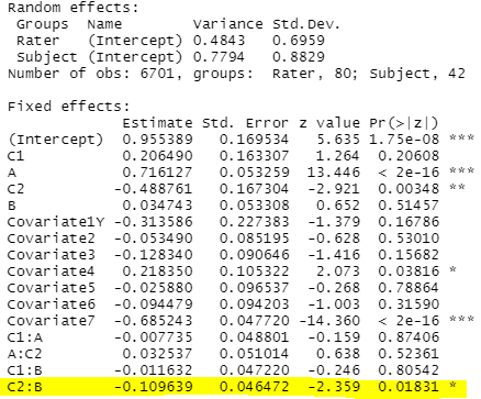
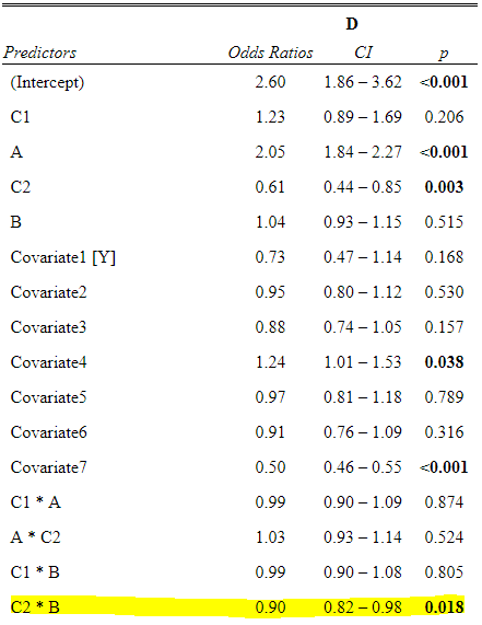
We fit a generalized model with A, B, and C as predictors of D, alongside covariates. We also included interactions between A and B and the linear and quadratic orthogonal polynomials for C (C1 and C2). Based on the model outputs summarized below, with the target interaction highlighted, the following appears to be true.

1. The relationship between B and D depends on C, as evidenced by the significant C2:B interaction. The fact that the coefficient is negative and the odds ratio < 1 suggests that at higher levels of C2, the relationship between B and D is negative, and at lower levels of C2, the relationship is positive. Because C2 is quadratic, it also indicates that the relationship between B and D is stronger at the extreme values of C2.

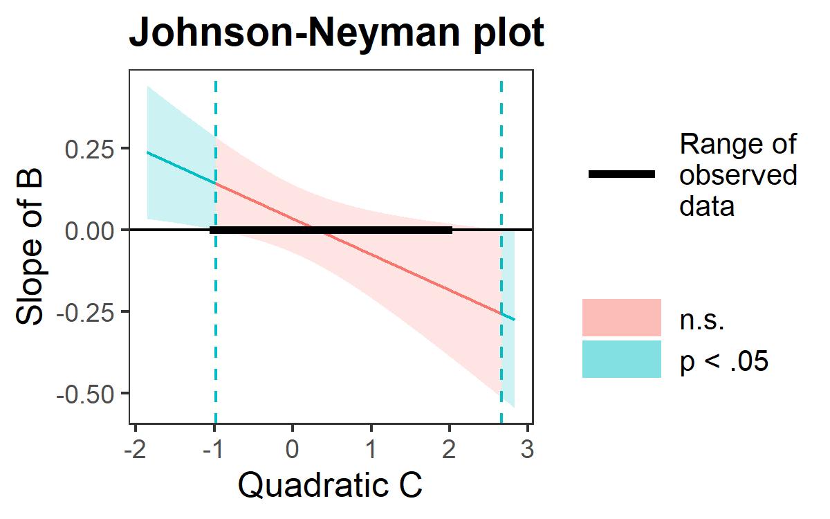
To visualize this effect, we used the johnson_neyman function of the interactions package. The plot shows how the relationship between B and D changes as a function of C2. The plot suggests that our interpretations of the interaction are correct. However, the plot also shows that the predicted significant relationships between B and D mostly fall outside of the range of observed values. Is there special language we should use when describing the interaction effect?

Code

#I'm having trouble generating sample data and copying it into the website (any tips would be helpful), so I'm limiting the sample code to the models and plots.
#Create orthogonal polynomials, increase scale width so that they are on the same standardized scale as the other predictors, and add them to the data set
#install.packages("polypoly") if needed
library(polypoly)
cv.data <- poly_add_columns(cv.data, C, 2, scale_width = 3)

#Fit and summarize the model
library(lme4)
fm.cv <- glmer(D ~ C1*A + C2*A + C1*B + C2*B + (1 | Subject) + (1 | Rater), family = binomial, data = cv.data)
summary(fm.cv)

#Generate odds ratio output
#install.packages("sjPlot") if needed
library(sjPlot)
tab_model(fm.cv)

#Create plot
library(ggplot2)
#install.packages("interactions") if needed
library(interactions)
jn <- johnson_neyman(model = fm.cv, pred = B, modx = C2)
plot.jn <- jn$plot + xlab("Quadratic C") + ylab("Slope of B")