Short

For the sake of the point of the book, you can interpret 'linear function' in the narrow sense as a polynomial function, or as ordinary least squares regression.

It is not about the semantics of what is or what is not a linear model. In this case the example is not a GLM (more about that below), but that is besides the point. Even if it would be GLM then it would be different from a polynomial function and the parameters $\phi_2$ and $\phi_3$ would have meaningful physical interpretations.

More than semantics

As Gordon Smyth mentions in the comments, it is more than just semantics. Due to the parameter $\phi_1$ the logistic growth model is not exactly equal to the logistic function used in logistic regression.

Compare

$$\phi_1/\lbrace 1+\text{exp}[-(t-\phi_2)/\phi_3]\rbrace$$

with

$$1/\lbrace 1+\text{exp}[-(t-\phi_2)/\phi_3]\rbrace$$

Logistic regression and fractions

Logistic regression deals with $\phi_1=1$. This relates to fractions between zero and one. The example from the book is a growth model and a different setting.

Not all fractions are logistic regression

Sidenote: I am saying that logistic regression relates to fractions, but not all fractions relate to logistic regression.

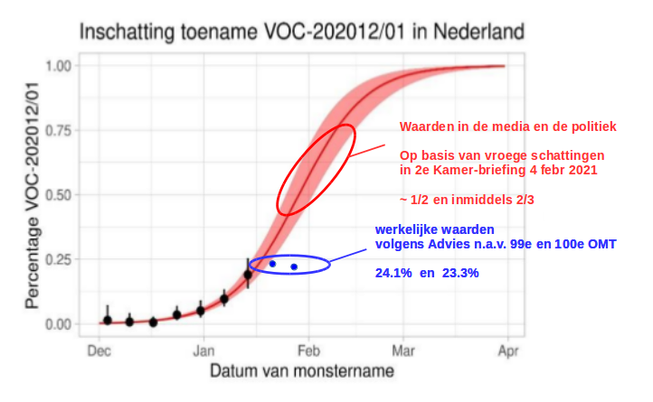
When we deal with fractions then we still might have $\phi_1 \neq 1$ for instance the fraction of coronavirus variants relates to growth models, and has been modeled by some with logistic curves that wrongly assume $\phi_1 = 1$.

An example is the forecasting of variants by the Dutch 'RijksInstituut Voor Veiligheid (RIVM)'. Besides problems with the exponential growth of the two different strains (leading to large discrepancies in the odds far beyond the prediction intervals) the model wrongly assumed $\phi_1 = 1$. In the picture below we see that this has the effect of unrealistic predictions for April, with statements that the fraction of infections with the variant is gonna be close to 1 with a very tiny error margin (the reality is that it is currently somewhere in the range 0.8 to 0.9).

For the growth model we can come up with ideas why the $\phi_1$ should not be equal to 1. Also for other models that deal with fractions it might be wrong as well. This is in particular problematic when the curves are fitted based on little data in a small range and subsequently extrapolated. This may contribute, for instance, to the piranha problem. Assuming linearity/addition of multiple effects on the log-odds can be problematic.

The semantics

What is a linear model?

Linearity is a broad term.

One might for instance consider it a model that is a straight line $a+bx$ or more general a matrix equation $\beta X$. But linearity could also relate to a function with the algebraic property $f(x+y) = f(x) + f(y)$ and $f(a\cdot x) = a\cdot f(x)$.

In statistics we have linear regression which makes the predictor a weighted sum of the observations (a linear function of the observations).

$\hat\beta = M \cdot y$

For instance OLS with $M = (X^TX)^{-1}X^T$ or ridge regression with $M = (X^TX -\lambda I)^{-1}X^T$.

Generalized linear models (GLMs) are not like that. You can not find $\hat\beta$ as a sum of the observations $y$, and instead will use some itterative method to approach the solution. But still, there is a linear aspect to GLM, which is that transformation (by means of the link function) of the conditional expectation of the data is a linear function of the regressors.

So yes GLM is in one way linear, but in another way it is not.

The illustration

The point of the book seems to be different from the semantic point, and is more about the idea that the ubiquitous ordinary least squares (linear) model, like a polynomial, might gonna fit the data well, but is different in interpretation. The coefficients can be meaningless (if the model is not mechanistic/ab-initio) and you can not rely on extrapolation.

(You wrote that you got the point, but this is just to be complete and help other bystanders/readers)

• Polynomials, splines, with or without some transform (as in GLM), or other general curves... they are often used as an empirical model and they have the advantage of being easy to fit.

• Non-linear models, they are often a mechanistic model and they have the disadvantage of being less easy to fit (but they are still used because of the greater interpretability and also they might be used for extrapolation to some extent).

The problem with the point of the book is that sometimes a (generalized) linear model can be a mechanistic model. The point is not about the idea whether the growth curve is a linear function or not (in some way or another), but about the idea that polynomials are often standard fitting methods without mechanistic meaning. The idea is that a non-polynomial function could be better. And whether this non-polynomial function is a GLM model that can still be interpreted as linear, or a non-linear model, that is besides the point.