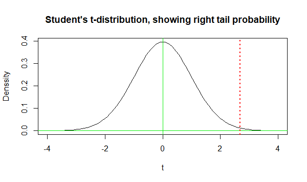
The answer by @Dave2e is fine (+1), but I wanted to give an Answer based mainly on a specific example and showing computations of P-values.
Consider the following fictitious data:
set.seed(2022)
x1 = rnorm(30, 350, 50)
x2 = rnorm(30, 300, 70)

summary(x1);  length(x1);  sd(x1)
   Min. 1st Qu.  Median    Mean 3rd Qu.    Max.
  205.0   309.6   346.7   344.2   379.2   410.6
[1] 30         # sample size
[1] 46.29298   # sample SD

summary(x2);  length(x2);  sd(x2)
   Min. 1st Qu.  Median    Mean 3rd Qu.    Max.
  190.9   281.3   310.5   307.6   353.5   418.5
[1] 30
[1] 58.53848
Now, do a two sample Welch t test of $H_0: \mu_1=\mu_2$
against $H_a: \mu_1 > \mu_2,$ using t.test in R:
t.test(x1,x2, alt="gr")

        Welch Two Sample t-test

data:  x1 and x2
t = 2.6864, df = 55.074, p-value = 0.004764
alternative hypothesis:
 true difference in means is greater than 0
95 percent confidence interval:
 13.8086     Inf
sample estimates:
mean of x mean of y
 344.2034  307.5991
The P-value of the test is computed by looking in the upper tail of Student's t distribution with 55.074 degrees of freedom. [DF is adjusted downward from $n_1+n_2-2=58$ to compensate for the difference in sample variances.]
1 - pt(2.6864, 55.074)
[1] 0.004764504
[In R, pt is a CDF of Student's t distribution.]
The P-value is the area under the density curve to the right of the vertical dotted red line.
R code for figure:
curve(dt(x, 55.074), -4, 4,
         ylab="Denssity", xlab="t", main=hdr)
 abline(h=0, col="green2")
 abline(v=0, col="green2")
 abline(h= 2.6864, col="red", lwd=2, lty="dotted")
 abline(v= 2.6864, col="red", lwd=2, lty="dotted")
If you do a 2-sided t test, then the P-value is calculated
by looking both in the lower tail below $-2.6864$ and in the upper tail above $2.6864.$ [By using $-notation, we show only the P-value.]
t.test(x1, x2)$p.val
[1] 0.009528523
This P-value for a 2-sided test is computed as follows:
pt(-2.6864, 55.074) + 1 - pt(2.6864, 55.074)
   # left tail + right tail
[1] 0.009529008
Alternatively, using the symmetry of the t distribution:
2*pt(-2.6864, 55.074)   $ Double left tail probability
[1] 0.009529008
Note: Quantities in the output of the test are rounded slightly to save space, so there is a tiny discrepancy with the P-values shown just above.
However, if you get confused (easy to do), and ask for the
wrong side, using parameter alt="less" in t.test, then
you get a nonsense P-value near $1.$
 t.test(x1, x2, alt="less")$p.val
 [1] 0.9952357

