I have a dataset like the following (n=1400):

register    country PC1
CMT BD  0.528902409041985
CMT IN  0.659599336404661
CMT LK  0.424746884028921
CMT PK  0.617481735398022
CMT UK  0.432241778651171
CMT US  0.520006978931032
TWT BD  -0.120412754435259
TWT IN  -0.775416939396557
TWT LK  -0.331060813776788
TWT PK  -0.0476004644598422
TWT UK  -0.751168065821314
TWT US  -0.861747850448701
TXM BD  -0.899207300872416
TXM IN  -1.90230790510253
TXM LK  0.257287440181
TXM PK  -1.3102770881823
WBF BD  -0.38312607807368
WBF IN  -1.4048106311512
WBF LK  -0.238559559698407
WBF PK  0.0249239934526432
WBF UK  -0.467017637887557
WBF US  -0.423802534509881
WBS BD  1.53739431443881
WBS IN  0.275786018712733
WBS LK  1.32988601584956
WBS PK  1.68224760320901
WBS UK  1.6017172088108
WBS US  1.34625059689434

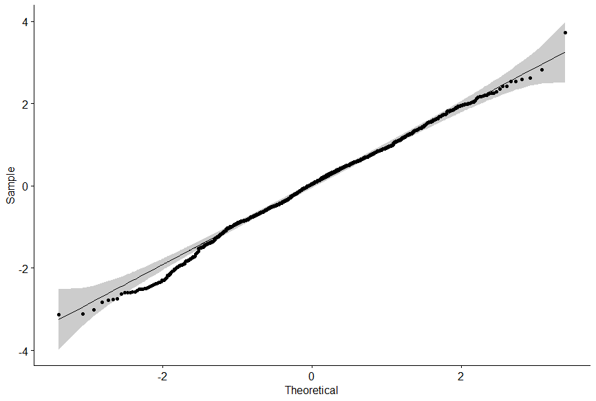
I am interested in ANOVA and if significant groups comparisons using emmeans package in R. The dependent variable PC1 is not normally distributed as per shapiro.test (p<0.001). See also qqplot below):

Which means that I cannot use anova() and emmeans in one go like this:

library(emmeans)
m_dims <- lm(PC1 ~ register*country, data = dims)
m_dims
anova(m_dims)
em_dims <- emmeans(m_dims, pairwise ~ country | register)

See the sample output:

Analysis of Variance Table

Response: PC1
                   Df Sum Sq Mean Sq  F value    Pr(>F)    
register            4 776.63 194.157 468.6266 < 2.2e-16 ***
country             5  20.55   4.111   9.9222 2.452e-09 ***
register:country   18  33.39   1.855   4.4769 1.411e-09 ***
Residuals        1372 568.43   0.414                       
---
Signif. codes:  0 ‘***’ 0.001 ‘**’ 0.01 ‘*’ 0.05 ‘.’ 0.1 ‘ ’ 1

And for emmeans()$contrasts (here only first two levels of register)

register = CMT:
 contrast estimate    SE   df t.ratio p.value
 BD - IN  -0.29759 0.129 1372  -2.312  0.1899
 BD - LK   0.42673 0.129 1372   3.315  0.0121
 BD - PK  -0.05777 0.129 1372  -0.449  0.9977
 BD - UK   0.07512 0.129 1372   0.584  0.9921
 BD - US   0.13296 0.129 1372   1.033  0.9069
 IN - LK   0.72432 0.129 1372   5.626  <.0001
 IN - PK   0.23981 0.129 1372   1.863  0.4257
 IN - UK   0.37271 0.129 1372   2.895  0.0445
 IN - US   0.43055 0.129 1372   3.344  0.0109
 LK - PK  -0.48451 0.129 1372  -3.764  0.0024
 LK - UK  -0.35161 0.129 1372  -2.731  0.0698
 LK - US  -0.29377 0.129 1372  -2.282  0.2021
 PK - UK   0.13290 0.129 1372   1.032  0.9071
 PK - US   0.19073 0.129 1372   1.482  0.6762
 UK - US   0.05783 0.129 1372   0.449  0.9977

register = TWT:
 contrast estimate    SE   df t.ratio p.value
 BD - IN  -0.38951 0.129 1372  -3.026  0.0303
 BD - LK  -0.13149 0.129 1372  -1.021  0.9109
 BD - PK  -0.12868 0.129 1372  -1.000  0.9182
 BD - UK   0.10248 0.129 1372   0.796  0.9682
 BD - US   0.34901 0.129 1372   2.711  0.0737
 IN - LK   0.25802 0.129 1372   2.004  0.3403
 IN - PK   0.26083 0.129 1372   2.026  0.3279
 IN - UK   0.49199 0.129 1372   3.822  0.0019
 IN - US   0.73852 0.129 1372   5.737  <.0001
 LK - PK   0.00281 0.129 1372   0.022  1.0000
 LK - UK   0.23397 0.129 1372   1.817  0.4547
 LK - US   0.48050 0.129 1372   3.733  0.0027
 PK - UK   0.23116 0.129 1372   1.796  0.4689
 PK - US   0.47769 0.129 1372   3.711  0.0029
 UK - US   0.24653 0.129 1372   1.915  0.3932

So I decided to use bootstrapping to resample my data, apply anova() and emmeans() on each sample and calculate the usual statistics for register, country, register*country: p-values, F statistic, degrees of freedom, R-sq etc. from anova() output, and pair wise comparisons of each country level (PK, UK, US, LK, IN, BD) within each register level (CMT, TWT, TXM, WBF, WBS). As per my very limited understanding of bootstrapping, I thought of averaging the resulting distributions to get each statistic, e.g. median p-value from all 1000 or more anova() outputs from my data samples. My questions:

1. Am I correct to assume that the p-value or any statistic obtained this way is a robust alternative to the one time output of anova() (or the subsequent emmeans()) as I showed above?
2. If my assumption is not correct, how should I proceed to apply bootstrap in this scenario? Before writing this post, I have consulted various blog posts and searched for ready-made solutions/functions in R but could not find anything suitable or convincing. Some references An R script for bootstrap ANOVA and post hoc comparisons. (I changed lsmeans to emmeans but it outputs same p-value for each post-hoc comparison which I do not understand why, so I left it). Bootstrap resampling with tidymodels Bootstrap Anova. Bootstrap followup contrasts (no ANOVA bootstrapping).