Return to Revisions

One way to do this will be profile likelihood. If we have a parameter vector $\psi$, profile likelihood is usually calculated for one of the components of $\psi$, but it can be defined for any parametric function of $\psi$. Below is a definition, suppose $L(\psi)$ is the likelihood function and interest (or focus) is on a scalar function $\theta = \theta(\psi)$, then $$ L_P(\theta) = \max_{\{\psi\colon \theta(\psi)=\theta \}} L(\psi)$$ The implementations of profile likelihood in R (elsewhere?) is not of these generality, so let us make it "by hand".

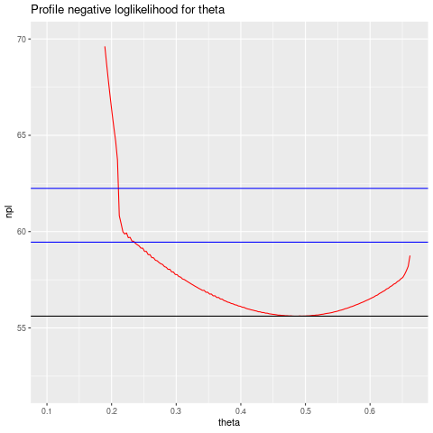
The model is $$ \DeclareMathOperator{\P}{\mathbb{P}} p_x= \P(Y=1 \mid X=x)= \frac1{1+e^{-\beta_0 - \beta_1 x}} $$ and the interest parameter $\theta$ is $$ \theta = p_{0.75} - p_{0.25} $$ It doesn't look promising to try to solve the optimization symbolically, so we try numerically. This is a first attempt, so maybe we can do better. First, a plot of the (negative) profile likelihood for $\theta$, using the data simulated in the question:

the two blue lines are cutoffs for confidence intervals of 95 and 99%, respectively, based on quantiles from the reference chi-square distribution with 1 df. R code is below:

### First run code from question
library(bbmle)

make_negloglik <- function(y, x) {
   n <- length(y)
   stopifnot( n == length(x) )
   Vectorize( function(beta0, beta1) 
       sum(ifelse(y==0, log1p(exp(beta0  +  beta1*x)),
                                   log1p(exp(-beta0 - beta1*x)))) )
    }

negloglik <- make_negloglik(y, x)

mod.bb <- bbmle::mle2(negloglik,  start=list(beta0=-2, beta1=4))

mod.prof <- bbmle::profile(mod.bb)

plot(mod.prof) # Not shown 

grid <- expand.grid(beta0=seq(-2.8, -0.5, len=100),
                    beta1=seq(1.8, 7.1, len=100))
grid$negloglik <-  with(grid, negloglik(beta0, beta1)) 

P <- function(beta0, beta1, x) 1/( 1  + exp( -beta0 -beta1 * x))

theta <- function(beta0, beta1) P(beta0, beta1, 0.75) - P(beta0, beta1, 0.25)

### Adding theta as a column to data.frame grid:

grid$theta <- with(grid, theta(beta0, beta1))

profile_negloglik <- function(grid) {
    rt <- with(grid,  range(theta))
    seq_theta <- seq(rt[1], rt[2], len=201)
    delta <- diff(seq_theta[1:2])
    npl <- numeric(length=length(seq_theta))
    for (t in seq_along(seq_theta)) {
        tt <- seq_theta[t]
        npl[t] <- with(grid, min(grid[ (tt-delta/2 <= theta) & (theta <= tt + delta/2),
                                      "negloglik" ]))
        }
    return(data.frame(theta=seq_theta, npl=npl))
    }

npl_frame <- profile_negloglik(grid)

npl_min <- with(npl_frame, min(npl))

library(ggplot2)

ggplot(npl_frame, aes(theta, npl))  +  geom_line(color="red")  +
    ggtitle("Profile negative loglikelihood for theta")  +
    geom_hline(yintercept=npl_min)  +
    geom_hline(yintercept=npl_min +  qchisq(0.95, 1), color="blue")  +
    geom_hline(yintercept=npl_min +  qchisq(0.99, 1), color="blue")   +
    ylim(52, 70)   

The idea of the code is:

• Define a rectangle in parameter space given by individual 99% confidence intervals (calculated by profiling with the R package bbmle)
• use expand.grid to cover the rectangle
• add to the grid data frame a column with the negative loglikelihood, another column with $\theta$
• Find the range of $\theta$ and subdivide it in many small intervals
• For each of the intervals, find the minimum negative log likelihood over the interval, and associate that with the midpoint
• finally, plot this as an approximation of the negative profile loglikelihood function of $\theta$. ggplot(npl_frame, aes(theta, npl)) + geom_line(color="red") + ggtitle("Profile negative loglikelihood for theta") + geom_hline(yintercept=npl_min) + geom_hline(yintercept=npl_min + qchisq(0.95, 1), color="blue") + geom_hline(yintercept=npl_min + qchisq(0.99, 1), color="blue") + ylim(52, 70)