The result may say the quadratic factor is statistically significant, but with a value is $10^{−14}$ it is physically insignificant.
I am thinking your question is "Why is there a quadratic coefficient so small and not equal to 0 from the original definition?" To answer this look at your plot. The x range (from 0 to 1) is small and in that range the function is linear. (no curvature). The contribution quadratic (or higher orders) is very small in the range of -1 < x < 1. Since the square of small number is even smaller. ) $.1^2 = 0.01$, thus no contribution.
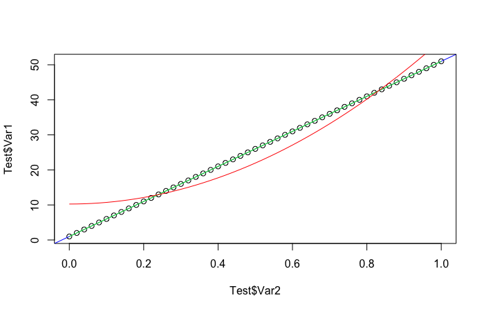
See the blue and green lines below. Both lines are nearly equal.
Now for your second model, fitting a quadratic without the linear term.
The least squares method is finding the best 2 coefficients to minimize the error and the result is the red curve. Again there are 50 data points in a small x-range where the quadratic effect is insignificant and thus still a pretty good linear fit.
In fact you just fit the intercept (without any independent variable) you will still end up with a decent fit.
Hopefully this help cleared up your confusion.
Var1 <- seq(1:51)
Var2 <- seq(0, 1, 0.02)
Var3 <- Var2^2
Test <- data.frame(cbind(Var1, Var2, Var3))
plot(Test$Var2, Test$Var1)

linear <- lm(Var1 ~ Var2, Test)
summary(linear)
abline(linear, col="blue")

quad <- lm(Var1 ~ Var2 + Var3, Test)
summary(quad)
lines(x=Test$Var2, y=predict(quad, Test), col="green")

quad_lite <- lm(Var1 ~ Var3, Test)
summary(quad_lite)
lines(x=Test$Var2, y=predict(quad_lite, Test), col="red")

intercept <- lm(Var1 ~ 1, Test)
summary(intercept)

