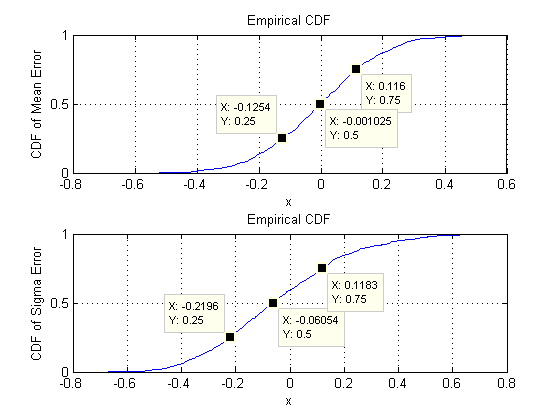
Some brief numerics gives the following error distributions for the fit of 30 samples created from a standard normal distribution then fit to a univariate Gaussian.

The quartiles are indicated. It is assumed that this level of variation is desired in the multi-dimensional case.
I don't have the time to beat up MatLab to get the total result, so I will share my "rule of thumb". The 30 is provided as a rule of thumb, or heuristic so it is assumed that heuristics are not unacceptable.
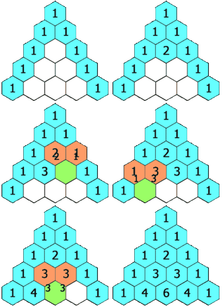
My heuristic is to use Pascals triangle multiplied by the univariate case.

If I am using 2d data then I go to the 2nd row and sum it to get 2x the number of samples, or 60 samples. For 3d data I go to the 3rd row and sum it to get 4x the number of samples or 120 samples. For 5d data I go to the 5th row and sum it to get 16x the number of samples, or 480 samples.
Best of luck.
EDit:
It was intuitve, but everything has to be defended in math. I can't just take leaps from formulation of polynomial forms from Finite Elements with experience to get a ballpark.
The equation for the sum of that row of Pascals triangle is 2^k.
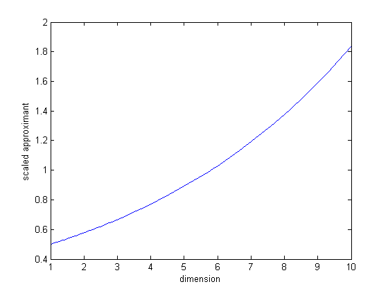
Using expression 2.88 in here with the multivariate Gaussian, taking the first functional variation and setting the mean and its variation to zero, then solving for the functional variation with respect to dimension yields the following general form: $ \delta k =A \log \left ( 2^k pi^k f(s)\right ) -k$. Observation shows all terms in the brackets are positive, so minimization of the interior is minimization of the functional. Though it is hand-wavy it can be argued that k is always positive, so it can be expressed as a log(exp(k)) and included as a denominator. When I look at this expression and divide it by $ 2^k$ and multiply it by $ \frac {e}{2\pi}$ as I sweep k from 1 to 10 I notice that the values is between 0.6 and 2. As an engineer where "good enough" makes a rule of thumb I can say that, to me this is a approximator for the first functional variation of the change in log-likelihood (with some simplifying assumptions about the mean) that allows me to relate expectation to dimension. Knowing this is a mean, I can then relate sample size to dimension.

The idea here is to use log-likelihood to relate the lower-dimensional distribution with fewer samples to the higher dimensional distribution with more samples.
The Akaike Information Criteria (AIC) is defined as $ AIC = n log(RSS/n) + 2*k$ where RSS is residual sum of squares, n is sample count, and k is parameter count for the model.
Setting the AIC between two distributions equal we get $ n_1 log(RSS_1/n_1) +2k_1 = n_2 log(RSS_2/n_2) +2k_2$. Each dimension we add to the space adds a row to the mean and a row and a column to the covariance. $k_2 = 2 k_1 +2$. Assuming the error per sample point is constant relates the residual sum of squares to the sample count, and the term in the logarithm stays constant. The difference in sample count becomes a scaling constant.
I am now looking at the z-transform in order to make this a more useful expression. (to be continued... possibly with AICc).
