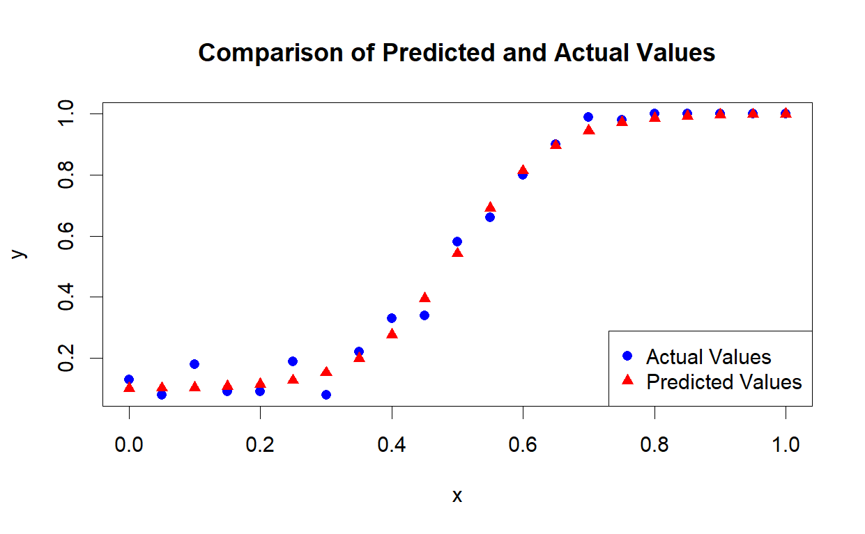
A quick workaround is to use nonlinear least squares estimation and bound the S-shaped curve to the (0.1,1) range.
# estimate the model with adjusted asymptotes
m1 <- nls(y ~ 0.1 + 0.9*exp(a+b*x)/(1 + exp(a+b*x)),
        start = list(a=0, b = 0))

# predict y
y_predicted = predict(m1, x)

# Plot the actual values with points only
plot(x, y, type = 'p', col = 'blue', pch = 16, xlab = 'x', ylab = 'y',
     main = 'Comparison of Predicted and Actual Values')

# Add the predicted values with points only
points(x, y_predicted, type = 'p', col = 'red', pch = 17)

# Add a legend to the plot
legend("bottomright", legend=c("Actual Values", "Predicted Values"),
       col=c("blue", "red"), pch=c(16, 17))

