You can test equality of the mean parameters against the alternative that the mean parameters are unequal with a likelihood ratio test. (However, if the mean parameters do differ and the distribution is exponential, this is a scale shift, not a location shift.)
Let's say we parameterize the $i$th observation in the first exponential as having pdf $1/\mu_x \exp(-x_i/\mu_x)$ and the $j$th observation in the second sample as having pdf $1/\mu_y \exp(-y_j/\mu_y)$ (over the obvious domains for the observations and parameters).
(To be clear, we're working in the mean-form not the rate-form here; this won't affect the outcome of the calculations.)
Since the distribution of $X_i$ is a special case of the gamma, $\Gamma(1,\mu_x)$, the distribution of the sum of $X$'s, $S_x$ is distributed $\Gamma(n_x,\mu_x)$; similarly that for the sum of the $Y$s, $S_y$ is $\Gamma(n_y,\mu_y)$.
Because of the relationship between gamma distributions and chi-squared distributions, it turns out that $2/\mu_x S_x$ is distributed $\chi^2_{2n_x}$. The ratio of two chi-squares on their degrees of freedom is F. Hence the ratio, $\frac{\mu_y}{\mu_x}\frac{S_x/n_x}{S_y/n_y} \sim F_{2n_x,2n_y}$.
Under the null hypothesis of equality of means, then, $\bar x/\bar y \sim F_{2n_x,2n_y}$, and under the two sided alternative, the values might tend to be either smaller or larger than a value from the null distribution, so you need a two-tailed test.
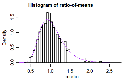
Simulation to check that we didn't make some simple mistake in the algebra:
Here I simulated 1000 samples of size 30 for $X$ and 20 for $Y$ from an exponential distribution with the same mean, and computed the above ratio-of-means statistic.
Below is a histogram of the resulting distribution as well as a curve showing the $F$ distribution we computed under the null:

Example, with discussion of computation of two-tailed p-values:
To illustrate the calculation, here's two small samples from exponential distributions. The X-sample has 14 observations with mean 10, the Y-sample has 17 observations with mean 15:
x: 12.173  3.148 33.873  0.160  3.054 11.579 13.491  7.048 48.836
   16.478  3.323  3.520  7.113  5.358

y:  7.635  1.508 29.987 13.636  8.709 13.132 12.141  5.280 23.447
   18.687 13.055 47.747  0.334  7.745 26.287 34.390  9.596
The ratio of means is 0.7515
The area to the left is straightforward, since it's in the lower tail (calc in R):
 > pf(r,28,34)
 [1] 0.2210767
We need the probability for the other tail. If the distribution was symmetric in the inverse, it would be straightforward to do this.
A common convention with the ratio of variances F-test (which is similarly two tailed) is simply to double the one-tailed p-value (effectively what is going on as here; that's also what seems to be done in R, for example); in this case it gives a p-value of 0.44.
However, if you do it with a formal rejection rule, by putting an area of $\alpha/2$ in each tail, you'd get critical values as described here. The p-value is then the largest $\alpha$ that would lead to rejection, which is equivalent to adding the one tailed p-value above to the one-tailed p-value in the other tail for the degrees of freedom interchanged. In the above example that gives a p-value of 0.43.
