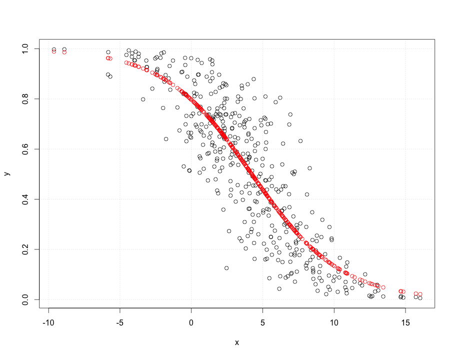
Given the skew in the data with x, the obvious first thing to do is use a logisitic regression (wiki link). So I am with whuber on this. I will say that $x$ on its own will show strong significance but not explain away most of the deviance (the equivalent of total sum of squares in an OLS). So one might suggest that there is another covariate apart from $x$ that aids explanatory power. Your $y$ data is already [0,1] though: do you know if they represent probabilities or occurrence ratios ? If so, you should try a logistic regression using your non-transformed $y$ (before they are ratios/probabilities).
Peter Flom's observation also makes sense given that y is already magically [0,1]. Check plot(density(y));rug(y) at different buckets of $x$ and see if you see a changing Beta distribution or simply run betareg. Note that the beta distribution is not an exponential family distribution and thus cannot be modeled with glm in R and you should use Peter's suggestion.
To give you an idea of what I meant by logistic regression:
# the 'real' relationship where y is interpreted as the probability of success
y = runif(400)
x = -2*(log(y/(1-y)) - 2) + rnorm(400,sd=2)
glm.logit=glm(y~x,family=binomial); summary(glm.logit)
plot(y ~ x); require(faraway); grid()
points(x,ilogit(coef(glm.logit) %*% rbind(1.0,x)),col="red")
tt=runif(400)  # an example of your untransformed regression
newy = ifelse(tt < y, 1, 0)
glm.logit=glm(newy~x,family=binomial); summary(glm.logit)

# if there is not a good match in your tail probabilities try different link function or oversampling with correction (will be worse here, but perhaps not in your data)
glm.probit=glm(y~x,family=binomial(link=probit)); summary(glm.probit)
glm.cloglog=glm(y~x,family=binomial(link=cloglog)); summary(glm.cloglog)

