Is PCA followed by a rotation (such as varimax) still PCA?

Question

I have tried to reproduce some research (using PCA) from SPSS in R. In my experience, principal() function from package psych was the only function that came close (or if my memory serves me right, dead on) to match the output. To match the same results as in SPSS, I had to use parameter principal(..., rotate = "varimax"). I have seen papers talk about how they did PCA, but based on the output of SPSS and use of rotation, it sounds more like Factor analysis.

Question: Is PCA, even after rotation (using varimax), still PCA? I was under the impression that this might be in fact Factor analysis... In case it's not, what details am I missing?

Answer 1

This question is largely about definitions of PCA/FA, so opinions might differ. My opinion is that PCA+varimax should not be called either PCA or FA, bur rather explicitly referred to e.g. as "varimax-rotated PCA".

I should add that this is quite a confusing topic. In this answer I want to explain what a rotation actually is; this will require some mathematics. A casual reader can skip directly to the illustration. Only then we can discuss whether PCA+rotation should or should not be called "PCA".

One reference is Jolliffe's book "Principal Component Analysis", section 11.1 "Rotation of Principal Components", but I find it could be clearer.

---

Let $\mathbf X$ be a $n \times p$ data matrix which we assume is centered. PCA amounts (see my answer here) to a singular-value decomposition: $\mathbf X=\mathbf{USV}^\top$. There are two equivalent but complimentary views on this decomposition: a more PCA-style "projection" view and a more FA-style "latent variables" view.

According to the PCA-style view, we found a bunch of orthogonal directions $\mathbf V$ (these are eigenvectors of the covariance matrix, also called "principal directions" or "axes"), and "principal components" $\mathbf{US}$ (also called principal component "scores") are projections of the data on these directions. Principal components are uncorrelated, the first one has maximally possible variance, etc. We can write: $$\mathbf X = \mathbf{US}\cdot \mathbf V^\top = \text{Scores} \cdot \text{Principal directions}.$$

According to the FA-style view, we found some uncorrelated unit-variance "latent factors" that give rise to the observed variables via "loadings". Indeed, $\widetilde{\mathbf U}=\sqrt{n-1}\mathbf{U}$ are standardized principal components (uncorrelated and with unit variance), and if we define loadings as $\mathbf L = \mathbf{VS}/\sqrt{n-1}$, then $$\mathbf X= \sqrt{n-1}\mathbf{U}\cdot (\mathbf{VS}/\sqrt{n-1})^\top =\widetilde{\mathbf U}\cdot \mathbf L^\top = \text{Standardized scores} \cdot \text{Loadings}.$$ (Note that $\mathbf{S}^\top=\mathbf{S}$.) Both views are equivalent. Note that loadings are eigenvectors scaled by the respective eigenvalues ($\mathbf{S}/\sqrt{n-1}$ are eigenvalues of the covariance matrix).

(I should add in brackets that PCA$\ne$FA; FA explicitly aims at finding latent factors that are linearly mapped to the observed variables via loadings; it is more flexible than PCA and yields different loadings. That is why I prefer to call the above "FA-style view on PCA" and not FA, even though some people take it to be one of FA methods.)

Now, what does a rotation do? E.g. an orthogonal rotation, such as varimax. First, it considers only $k<p$ components, i.e.: $$\mathbf X \approx \mathbf U_k \mathbf S_k \mathbf V_k^\top = \widetilde{\mathbf U}_k \mathbf L^\top_k.$$ Then it takes a square orthogonal $k \times k$ matrix $\mathbf T$, and plugs $\mathbf T\mathbf T^\top=\mathbf I$ into this decomposition: $$\mathbf X \approx \mathbf U_k \mathbf S_k \mathbf V_k^\top = \mathbf U_k \mathbf T \mathbf T^\top \mathbf S_k \mathbf V_k^\top = \widetilde{\mathbf U}_\mathrm{rot} \mathbf L^\top_\mathrm{rot},$$ where rotated loadings are given by $\mathbf L_\mathrm{rot} = \mathbf L_k \mathbf T$, and rotated standardized scores are given by $\widetilde{\mathbf U}_\mathrm{rot} = \widetilde{\mathbf U}_k \mathbf T$. (The purpose of this is to find $\mathbf T$ such that $\mathbf L_\mathrm{rot}$ became as close to being sparse as possible, to facilitate its interpretation.)

Note that what is rotated are: (1) standardized scores, (2) loadings. But not the raw scores and not the principal directions! So the rotation happens in the latent space, not in the original space. This is absolutely crucial.

From the FA-style point of view, nothing much happened. (A) The latent factors are still uncorrelated and standardized. (B) They are still mapped to the observed variables via (rotated) loadings. (C) The amount of variance captured by each component/factor is given by the sum of squared values of the corresponding loadings column in $\mathbf L_\mathrm{rot}$. (D) Geometrically, loadings still span the same $k$-dimensional subspace in $\mathbb R^p$ (the subspace spanned by the first $k$ PCA eigenvectors). (E) The approximation to $\mathbf X$ and the reconstruction error did not change at all. (F) The covariance matrix is still approximated equally well:$$\boldsymbol \Sigma \approx \mathbf L_k\mathbf L_k^\top = \mathbf L_\mathrm{rot}\mathbf L_\mathrm{rot}^\top.$$

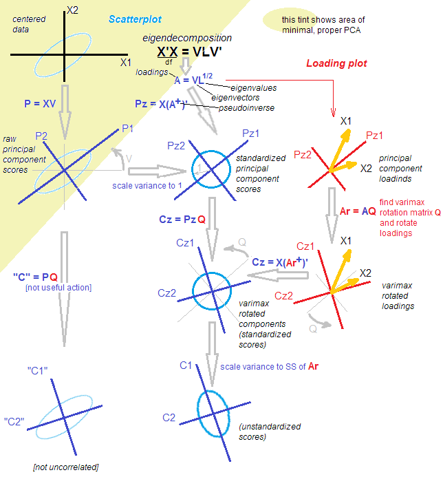
But the PCA-style point of view has practically collapsed. Rotated loadings do not correspond to orthogonal directions/axes in $\mathbb R^p$ anymore, i.e. columns of $\mathbf L_\mathrm{rot}$ are not orthogonal! Worse, if you [orthogonally] project the data onto the directions given by the rotated loadings, you will get correlated (!) projections and will not be able to recover the scores. [Instead, to compute the standardized scores after rotation, one needs to multiply the data matrix with the pseudo-inverse of loadings $\widetilde{\mathbf U}_\mathrm{rot} = \mathbf X (\mathbf L_\mathrm{rot}^+)^\top$. Alternatively, one can simply rotate the original standardized scores with the rotation matrix: $\widetilde{\mathbf U}_\mathrm{rot} = \widetilde{\mathbf U} \mathbf T$.] Also, the rotated components do not successively capture the maximal amount of variance: the variance gets redistributed among the components (even though all $k$ rotated components capture exactly as much variance as all $k$ original principal components).

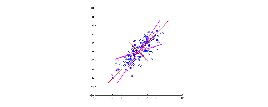
Here is an illustration. The data is a 2D ellipse stretched along the main diagonal. First principal direction is the main diagonal, the second one is orthogonal to it. PCA loading vectors (eigenvectors scaled by the eigenvalues) are shown in red -- pointing in both directions and also stretched by a constant factor for visibility. Then I applied an orthogonal rotation by $30^\circ$ to the loadings. Resulting loading vectors are shown in magenta. Note how they are not orthogonal (!).

An FA-style intuition here is as follows: imagine a "latent space" where points fill a small circle (come from a 2D Gaussian with unit variances). These distribution of points is then stretched along the PCA loadings (red) to become the data ellipse that we see on this figure. However, the same distribution of points can be rotated and then stretched along the rotated PCA loadings (magenta) to become the same data ellipse.

[To actually see that an orthogonal rotation of loadings is a rotation, one needs to look at a PCA biplot; there the vectors/rays corresponding to original variables will simply rotate.]

---

Let us summarize. After an orthogonal rotation (such as varimax), the "rotated-principal" axes are not orthogonal, and orthogonal projections on them do not make sense. So one should rather drop this whole axes/projections point of view. It would be weird to still call it PCA (which is all about projections with maximal variance etc.).

From FA-style point of view, we simply rotated our (standardized and uncorrelated) latent factors, which is a valid operation. There are no "projections" in FA; instead, latent factors generate the observed variables via loadings. This logic is still preserved. However, we started with principal components, which are not actually factors (as PCA is not the same as FA). So it would be weird to call it FA as well.

Instead of debating whether one "should" rather call it PCA or FA, I would suggest to be meticulous in specifying the exact used procedure: "PCA followed by a varimax rotation".

---

Postscriptum. It is possible to consider an alternative rotation procedure, where $\mathbf{TT}^\top$ is inserted between $\mathbf{US}$ and $\mathbf V^\top$. This would rotate raw scores and eigenvectors (instead of standardized scores and loadings). The biggest problem with this approach is that after such a "rotation", scores will not be uncorrelated anymore, which is pretty fatal for PCA. One can do it, but it is not how rotations are usually being understood and applied.

Answer 2

Principal Components Analysis (PCA) and Common Factor Analysis (CFA) are distinct methods. Often, they produce similar results and PCA is used as the default extraction method in the SPSS Factor Analysis routines. This undoubtedly results in a lot of confusion about the distinction between the two.

The bottom line is, these are two different models, conceptually. In PCA, the components are actual orthogonal linear combinations that maximize the total variance. In FA, the factors are linear combinations that maximize the shared portion of the variance--underlying "latent constructs". That's why FA is often called "common factor analysis". FA uses a variety of optimization routines and the result, unlike PCA, depends on the optimization routine used and starting points for those routines. Simply there is not a single unique solution.

In R, the factanal() function provides CFA with a maximum likelihood extraction. So, you shouldn't expect it to reproduce an SPSS result which is based on a PCA extraction. It's simply not the same model or logic. I'm not sure if you would get the same result if you used SPSS's Maximum Likelihood extraction either as they may not use the same algorithm.

For better or for worse in R, you can, however, reproduce the mixed up "factor analysis" that SPSS provides as its default. Here's the process in R. With this code, I'm able to reproduce the SPSS Principal Component "Factor Analysis" result using this dataset. (With the exception of the sign, which is indeterminant). That result could also then be rotated using any of Rs available rotation methods.

# Load the base dataset attitude to work with.
data(attitude)
# Compute eigenvalues and eigen vectors of the correlation matrix.
pfa.eigen<-eigen(cor(attitude))
# Print and note that eigen values are those produced by SPSS.
# Also note that SPSS will extract 2 components as eigen values > 1 = 2
pfa.eigen$values
# set a value for the number of factors (for clarity)
factors<-2
# Extract and transform two components.
pfa.eigen$vectors [ , 1:factors ]  %*% 
+ diag ( sqrt (pfa.eigen$values [ 1:factors ] ),factors,factors )

Answer 3

This answer is to present, in a path chart form, things about which @amoeba reasoned in his deep (but slightly complicated) answer on this thread (I'm a kind of agree with it by 95%) and how they appear to me.

PCA in its proper, minimal form is the specific orthogonal rotation of correlated data to its uncorrelated form, with the principal components skimming sequentially less and less of the overall variability. If the dimensionality reduction is all we want we usually don't compute loadings and whatever they drag after them. We're happy with the (raw) principal component scores $\bf P$. [Please note that notations on the chart don't precisely follow @amoeba's, - I stick to what I adopt in some of my other answers.]

On the chart, I take a simple example of two variables p=2 and use both extracted principal components. Though we usually keep only few first m<p components, for the theoretical question we're considering ("Is PCA with rotation a PCA or what?") it makes no difference if to keep m or all p of them; at least in my particular answer.

The trick of loadings is to pull scale (magnitude, variability, inertia $\bf L$) off the components (raw scores) and onto the coefficients $\bf V$ (eigenvectors) leaving the former to be bare "framework" $\bf P_z$ (standardized pr. component scores) and the latter to be fleshy $\bf A$ (loadings). You restore the data equally well with both: $\bf X=PV'=P_zA'$. But loadings open prospects: (i) to interpret the components; (ii) to be rotated; (iii) to restore correlations/covariances of the variables. This is all due to the fact that the variability of the data has been written in loadings, as their load.

And they can return that load back to the data points any time - now or after rotation. If we conceive of an orthogonal rotation such as varimax that means that we want the components to remain uncorrelated after the rotation done. Only data with spherical covariance matrix, when rotated orthogonally, preserves uncorrelatedness. And voila, the standardized principal components (which in machine learning often are called "PCA-whitened data") $\bf P_z$ are that magic data ($\bf P_z$ are actually proportional to the left, i.e. row eigenvectors of the data). While we are in search of the varimax rotation matrix $\bf Q$ to facilitate interpretation of loadings the data points passively await in their chaste sphericity & identity (or "whiteness").

After $\bf Q$ is found, rotation of $\bf P_z$ by it is equivalent to usual way computation of standardized principal component scores via the generalized inverse of the loading matrix, - this time, of the rotated loadings, $\bf A_r$ (see the chart). The resultant varimax-rotated principal components, $\bf C_z$ are uncorrelated, like we wanted it, plus data are restored by them as nicely as before rotation: $\bf X=P_zA'=C_zA_r'$. We may then give them back their scale deposited (and accordingly rotated) in $\bf A_r$ - to unstandardize them: $\bf C$.

We should be aware, that "varimax-rotated principal components" are not principal components anymore: I used notation Cz, C, instead of Pz, P, to stress it. They are just "components". Principal components are unique, but components can be many. Rotations other than varimax will yield other new variables also called components and also uncorrelated, besides our $\bf C$ ones.

Also to say, varimax-rotated (or otherwise orthogonally rotated) principal components (now just "components"), while remain uncorrelated, orthogonal, do not imply that their loadings are also still orthogonal. Columns of $\bf A$ are mutually orthogonal (as were eigenvectors $\bf V$), but not columns of $\bf A_r$ (see also footnote here).

And finally - rotating raw principal components $\bf P$ with our $\bf Q$ isn't useful action. We'll get some correlated varibles $\bf "C"$ with problematic meaning. $\bf Q$ appeared as to optimize (in some specific way) the configuration of loadings which had absorbed all the scale into them. $\bf Q$ was never trained to rotate data points with all the scale left on them. The rotating $\bf P$ with $\bf Q$ will be equivalent to rotating eigenvectors $\bf V$ with $\bf Q$ (into $\bf V_r$) and then computing the raw component scores as $\bf "C"=XV_r$. These "paths" noted by @amoeba in their Postscriptum.

These lastly outlined actions (pointless for the most part) remind us that eigenvectors, not only loadings, could be rotated, in general. For example, varimax procedure could be applied to them to simplify their structure. But since eigenvectors are not as helpful in interpreting the meaning of the components as the loadings are, rotation of eigenvectors is rarely done.

So, PCA with subsequent varimax (or other) rotation is

• still PCA
• which on the way abandoned principal components for just components
• that are potentially more (than the PCs) interpretable as "latent traits"
• but were not modeled satistically as those (PCA is not fair factor analysis)

I did not refer to factor analysis in this answer. It seems to me that @amoeba's usage of word "latent space" is a bit risky in the context of the question asked. I will, however, concur that PCA + analytic rotation might be called "FA-style view on PCA".

Answer 4

In psych::principal() you can do different types of rotations/transformations to your extracted Principal Component(s) or ''PCs'' using the rotate= argument, like: "none", "varimax" (Default), "quatimax", "promax", "oblimin", "simplimax", and "cluster". You have to empirically decide which one should make sense in your case, if needed, depending on your own appraisal and knowledge of the subject matter under investigation. A key question which might give you a hint: which one is more interpretable (again if needed)?

In the help you might find the following also helpful:

It is important to recognize that rotated principal components are not principal components (the axes associated with the eigen value decomposition) but are merely components. To point this out, unrotated principal components are labelled as PCi, while rotated PCs are now labeled as RCi (for rotated components) and obliquely transformed components as TCi (for transformed components). (Thanks to Ulrike Gromping for this suggestion.)

Answer 5

My understanding is that the distinction between PCA and Factor analysis primarily is in whether there is an error term. Thus PCA can, and will, faithfully represent the data whereas factor analysis is less faithful to the data it is trained on but attempts to represent underlying trends or communality in the data. Under a standard approach PCA is not rotated, but it is mathematically possible to do so, so people do it from time to time. I agree with the commenters in that the "meaning" of these methods is somewhat up for grabs and that it probably is wise to be sure the function you are using does what you intend - for example, as you note R has some functions that perform a different sort of PCA than users of SPSS are familiar with.

Answer 6

Thanks to the chaos in definitions of both they are effectively a synonyms. Don't believe words and look deep into the docks to find the equations.

Answer 7

Although this question has already an accepted answer I'd like to add something to the point of the question.

"PCA" -if I recall correctly - means "principal components analysis"; so as long as you're analyzing the principal components, may it be without rotation or with rotation, we are still in the analysis of the "principal components" (which were found by the appropriate initial matrix-decomposition).

I'd formulate that after "varimax"-rotation on the first two principal components, that we have the "varimax-solution of the two first pc's" (or something else), but still are in the framework of analysis of principal components, or shorter, are in the framework of "pca".

To make my point even clearer: I don't feel that the simple question of rotation introduces the problem of distinguishing between EFA and CFA (the latter mentioned /introduced into the problem for instance in the answer of Brett)

Answer 8

I found this to be the most helpful: Abdi & Williams, 2010, Principal component analysis.

ROTATION

After the number of components has been determined, and in order to facilitate the interpretation, the analysis often involves a rotation of the components that were retained [see, e.g., Ref 40 and 67, for more details]. Two main types of rotation are used: orthogonal when the new axes are also orthogonal to each other, and oblique when the new axes are not required to be orthogonal. Because the rotations are always performed in a subspace, the new axes will always explain less inertia than the original components (which are computed to be optimal). However, the part of the inertia explained by the total subspace after rotation is the same as it was before rotation (only the partition of the inertia has changed). It is also important to note that because rotation always takes place in a subspace (i.e., the space of the retained components), the choice of this subspace strongly influences the result of the rotation. Therefore, it is strongly recommended to try several sizes for the subspace of the retained components in order to assess the robustness of the interpretation of the rotation. When performing a rotation, the term loadings almost always refer to the elements of matrix Q.

(see paper for definition of Q).