Well, here is one but I will not prove it, only show it in simulation.
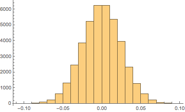
Make two beta distributions with equal large shape parameters $\text{Beta}(200,200)$ (here, $n=40,000$), subtract 1/2 from the $x$-values of one of them and call it "numerator." That gives us a PDF that has a maximum range of $\left(-\frac{1}{2},\,\frac{1}{2}\right)$, but because the shape parameters are so large, we never get to the maximum values of the range. Here is a histogram of an $n=40,000$ "numerator"

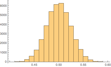
Next, we call the second beta distribution "denominator" without subtracting anything, so it has the usual beta distribution range of $(0,1)$ and one of those looks like this

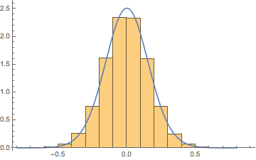
Again, because the shapes are so large, we do not approach the maximum range with the values. Next we plot the quotient $\frac{\text{numerator}}{\text{denominator}}$ as a PDF with the superimposed normal distribution.

Now in this case the normal distribution result has $\mu \to -0.0000204825,\sigma \to 0.0501789$ and tests for normality that look like this
$$\left(
\begin{array}{ccc}
\text{} & \text{Statistic} & \text{P-Value} \\
\text{Anderson-Darling} & 0.799786 & 0.481181 \\
\text{Baringhaus-Henze} & 1.40585 & 0.0852017 \\
\text{Cramér-von Mises} & 0.123145 & 0.482844 \\
\text{Jarque-Bera ALM} & 4.48103 & 0.106404 \\
\text{Kolmogorov-Smirnov} & 0.00452328 & 0.386335 \\
\text{Kuiper} & 0.00798063 & 0.109127 \\
\text{Mardia Combined} & 4.48103 & 0.106404 \\
\text{Mardia Kurtosis} & 1.53849 & 0.123929 \\
\text{Mardia Skewness} & 2.09399 & 0.147879 \\
\text{Pearson }\chi ^2 & 134.353 & 0.571925 \\
\text{Watson }U^2 & 0.113831 & 0.211187 \\
\end{array}
\right)$$
In other words, we cannot prove the ratio is not normal even trying very hard to do so.
Now why? Intuition on my part, which I have in overabundance. Proof left to reader, if any exists (maybe via limit of method of moments, but again that is just intuition).
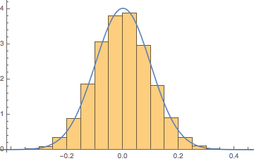
Hint: If I use only $\text{Beta}(20,20)$ in denominator and $\text{Beta}(20,20)-\frac{1}{2}$ in the numerator and I get Student's $t$ with $\mu \to -0.000251208,\sigma \to 0.157665,\text{df}\to 33.0402$

$$\begin{array}{l|ll}
\text{} & \text{Statistic} & \text{P-Value} \\
\hline
\text{Anderson-Darling} & 0.275262 & 0.955502 \\
\text{Cramér-von Mises} & 0.0351108 & 0.956524 \\
\text{Kolmogorov-Smirnov} & 0.00320936 & 0.804486 \\
\text{Kuiper} & 0.00556501 & 0.657146 \\
\text{Pearson }\chi ^2 & 145.077 & 0.323168 \\
\text{Watson }U^2 & 0.0351042 & 0.878202 \\
\end{array}$$
Another hint $\dfrac{\mathcal{N}(0,1)}{\mathcal{N}(10,1/1000)}\to$ Student's $t$ $\mu \to -0.0000535722,\sigma \to 0.0992765,\text{df}\to 244.154$

$$\left(
\begin{array}{ccc}
\text{} & \text{Statistic} & \text{P-Value} \\
\text{Anderson-Darling} & 0.501677 & 0.745102 \\
\text{Cramér-von Mises} & 0.0696824 & 0.753515 \\
\text{Kolmogorov-Smirnov} & 0.00355688 & 0.692225 \\
\text{Kuiper} & 0.00608382 & 0.501133 \\
\text{Pearson }\chi ^2 & 142.88 & 0.370552 \\
\text{Watson }U^2 & 0.0603207 & 0.590369 \\
\end{array}
\right)$$
Edit "Under certain conditions a normal approximation is possible" See link. Moreover, the main text of that Wikipedia article shows interesting material on the ratio distribution topic. Another reference.

