I don't think this question has a clear statistical answer. It will come down to your particular requirements.

Think about the question each calculation answers. The first calculation, the variance of all task lengths, answers the question:

How much variation do we observe among all task lengths?

The second calculation answers a different question:

How much variation do we observe among the longest-running tasks?

The former gives a sense of overall spread. The latter gives a sense of spread in the upper tail. That is, it's a rough way of looking at the length of that tail. I say "rough" because it's delineated by an arbitrary cutoff — in this case the 90th percentile — and because there are probably more precise and targeted ways to measure tail length.

You can see how this works with some simulated data (in R):

N <- 10000
x <- rnorm(N)
y <- rt(N, 5)
boxplot(x, y, xaxt = "n")
abline(h = quantile(x, 0.9), col = "red")
abline(h = quantile(y, 0.9), col = "blue")
legend("bottom", paste("90th percentile: ", c("x", "y")), col = c("red", "blue"), lwd = 1)
var_90_pct <- function (x) var(x[x > quantile(x, 0.9)])
axis(1, 1:2, c("X: N(0,1)", "Y: T(5)"))
axis(1, 1:2, sprintf("90 pctile var = %.2f", c(var_90_pct(x), var_90_pct(y))), line = 2, tick = FALSE)
title(main = "Simulated Gaussian and Student t distributions\nwith 90th percentiles highlighted")

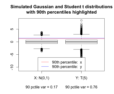
The Student t distribution (with few degrees of freedom) is distinguished from the standard Gaussian by its long tail. It is easy see on the graph that the Student t has much greater variance among the 10% of observations, despite the 90th percentiles themselves being very close together.

This is why I don't think the question has a clear answer. Which one do you actually care about? Maybe if you are comfortable with the running time of your 90th percentile tasks but are concerned about a few extreme cases, the "tail-only variance" might be good to study. Variance is pretty cheap to compute; honestly you should probably just do both. And consider graphing the data while you're at it.

I don't think this question has a clear statistical answer. It will come down to your particular requirements.

Think about the question each calculation answers. The first calculation, the variance of all task lengths, answers the question:

How much variation do we observe among all task lengths?

The second calculation answers a different question:

How much variation do we observe among the longest-running tasks?

The former gives a sense of overall spread. The latter gives a sense of spread in the upper tail. That is, it's a rough way of looking at the length of that tail. I say "rough" because it's delineated by an arbitrary cutoff — in this case the 90th percentile — and because there are probably more precise and targeted ways to measure tail length.

You can see how this works with some simulated data (in R):

N <- 10000
x <- rnorm(N)
y <- rt(N, 5)
boxplot(x, y, xaxt = "n")
abline(h = quantile(x, 0.9), col = "red")
abline(h = quantile(y, 0.9), col = "blue")
legend("bottom", paste("90th percentile: ", c("x", "y")), col = c("red", "blue"), lwd = 1)
var_90_pct <- function (x) var(x[x > quantile(x, 0.9)])
axis(1, 1:2, c("X: N(0,1)", "Y: T(5)"))
axis(1, 1:2, sprintf("90 pctile var = %.2f", c(var_90_pct(x), var_90_pct(y))), line = 2, tick = FALSE)
title(main = "Simulated Gaussian and Student t distributions\nwith 90th percentiles highlighted")

The Student t distribution (with few degrees of freedom) is distinguished from the standard Gaussian by its long tail. It is easy see on the graph that the Student t has much greater variance among the top 10% of observations, despite the 90th percentiles themselves being very close together.

This is why I don't think the question has a clear answer. Which one do you actually care about? Maybe if you are comfortable with the running time of your 90th percentile tasks but are concerned about a few extreme cases, the "tail-only variance" might be good to study. Variance is pretty cheap to compute; honestly you should probably just do both. And consider graphing the data while you're at it.

Edit: I should mention that overall variance will also reveal long-tailed-ness. But it is more likely to be affected by other features of the distribution like multimodality, whereas the 90th percentile variance is probably going to be more focused.