I revamped the example to give more information about prediction values and made some minor changes to the code.
Source Link

You can accomplish this with the effects package. Now, for a reproducible example:

library(nnet)

set.seed(892)

x <- c(rnorm(100, 10, 1))

y <- factor(rep_len(1:3, 100))

fit <- multinom(y ~ x)

That's the model, now let's get some predicted probabilities.

library(effects)

fit.eff <- effectEffect("x", fit)
data.frame(fit.eff$prob, fit.eff$lower.$model.matrix, fit.eff$prob, fit.eff$uppereff$lower.prob, 
           fit.eff$upper.prob)

  X.Intercept.  x   prob.X1   prob.X2   prob.X3 L.prob.X1  L.prob.X2 L.prob.X3 U.prob.X1 U.prob.X2 U.prob.X3
1            1  8 0.4211010 0.1119309 0.4669680 0.2218766 0.03696574 0.2565056 0.6498212 0.2927143 0.6898823
2            1  9 0.3962450 0.1958841 0.4078709 0.2704241 0.10428467 0.2805946 0.5374796 0.3376147 0.5488354
3            1 10 0.3478412 0.3198070 0.3323518 0.2583849 0.23216366 0.2442887 0.4494968 0.4223378 0.4339321
4            1 11 0.2780225 0.4753991 0.2465784 0.1689652 0.33171768 0.1449846 0.4217471 0.6232722 0.3871286

Which gives the probabilities for factor "1" in X, prob.X1, its lower confidence interval L.prob.X1 and its upper interval U.prob.X1.

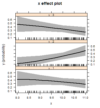
effects will helpfully plot the values for you as well, which is its main purpose anyway.

plot(fit.eff)
Edit: added some code to clarify which levels of x were being predicted. Note that Effect() automatically cuts numerical predictor variables based on grid.pretty, which might not be what you typically want. In this case, you need to set the xlevels option, like this: fit.eff <- effect("x", fit, xlevels = list(x = c(2, 4, 6, 8, 10))).

You can accomplish this with the effects package. Now, for a reproducible example:

library(nnet)

set.seed(892)

x <- c(rnorm(100, 10, 1))

y <- factor(rep_len(1:3, 100))

fit <- multinom(y ~ x)

That's the model, now let's get some predicted probabilities.

library(effects)

fit.eff <- effect("x", fit)
data.frame(fit.eff$prob, fit.eff$lower.prob, fit.eff$upper.prob)

    prob.X1   prob.X2   prob.X3 L.prob.X1  L.prob.X2 L.prob.X3 U.prob.X1 U.prob.X2 U.prob.X3
1 0.4211010 0.1119309 0.4669680 0.2218766 0.03696574 0.2565056 0.6498212 0.2927143 0.6898823
2 0.3962450 0.1958841 0.4078709 0.2704241 0.10428467 0.2805946 0.5374796 0.3376147 0.5488354
3 0.3478412 0.3198070 0.3323518 0.2583849 0.23216366 0.2442887 0.4494968 0.4223378 0.4339321
4 0.2780225 0.4753991 0.2465784 0.1689652 0.33171768 0.1449846 0.4217471 0.6232722 0.3871286

Which gives the probabilities for factor "1" in X, prob.X1, its lower confidence interval L.prob.X1 and its upper interval U.prob.X1.

effects will helpfully plot the values for you as well, which is its main purpose anyway.

plot(fit.eff)

You can accomplish this with the effects package. Now, for a reproducible example:

library(nnet)

set.seed(892)

x <- c(rnorm(100, 10, 1))

y <- factor(rep_len(1:3, 100))

fit <- multinom(y ~ x)

That's the model, now let's get some predicted probabilities.

fit.eff <- Effect("x", fit)
data.frame(fit.eff$model.matrix, fit.eff$prob, fit.eff$lower.prob, 
           fit.eff$upper.prob)

  X.Intercept.  x   prob.X1   prob.X2   prob.X3 L.prob.X1  L.prob.X2 L.prob.X3 U.prob.X1 U.prob.X2 U.prob.X3
1            1  8 0.4211010 0.1119309 0.4669680 0.2218766 0.03696574 0.2565056 0.6498212 0.2927143 0.6898823
2            1  9 0.3962450 0.1958841 0.4078709 0.2704241 0.10428467 0.2805946 0.5374796 0.3376147 0.5488354
3            1 10 0.3478412 0.3198070 0.3323518 0.2583849 0.23216366 0.2442887 0.4494968 0.4223378 0.4339321
4            1 11 0.2780225 0.4753991 0.2465784 0.1689652 0.33171768 0.1449846 0.4217471 0.6232722 0.3871286

Which gives the probabilities for factor "1" in X, prob.X1, its lower confidence interval L.prob.X1 and its upper interval U.prob.X1.

effects will helpfully plot the values for you as well, which is its main purpose anyway.

plot(fit.eff)

Edit: added some code to clarify which levels of x were being predicted. Note that Effect() automatically cuts numerical predictor variables based on grid.pretty, which might not be what you typically want. In this case, you need to set the xlevels option, like this: fit.eff <- effect("x", fit, xlevels = list(x = c(2, 4, 6, 8, 10))).

Source Link

You can accomplish this with the effects package. Now, for a reproducible example:

library(nnet)

set.seed(892)

x <- c(rnorm(100, 10, 1))

y <- factor(rep_len(1:3, 100))

fit <- multinom(y ~ x)

That's the model, now let's get some predicted probabilities.

library(effects)

fit.eff <- effect("x", fit)
data.frame(fit.eff$prob, fit.eff$lower.prob, fit.eff$upper.prob)

    prob.X1   prob.X2   prob.X3 L.prob.X1  L.prob.X2 L.prob.X3 U.prob.X1 U.prob.X2 U.prob.X3
1 0.4211010 0.1119309 0.4669680 0.2218766 0.03696574 0.2565056 0.6498212 0.2927143 0.6898823
2 0.3962450 0.1958841 0.4078709 0.2704241 0.10428467 0.2805946 0.5374796 0.3376147 0.5488354
3 0.3478412 0.3198070 0.3323518 0.2583849 0.23216366 0.2442887 0.4494968 0.4223378 0.4339321
4 0.2780225 0.4753991 0.2465784 0.1689652 0.33171768 0.1449846 0.4217471 0.6232722 0.3871286

Which gives the probabilities for factor "1" in X, prob.X1, its lower confidence interval L.prob.X1 and its upper interval U.prob.X1.

effects will helpfully plot the values for you as well, which is its main purpose anyway.

plot(fit.eff)