Fitting data to an equation without free parameters
First, let's clarify what it means "to see how well my data fits to the equation" when you have a fixed equation as in your original question. You have data on $x$ and $y$, and your equation:
$$y=(3.5-(x/10))(x/25)^{5/2}$$
has no free parameters. Here's a plot; data points are circles, the equation a solid curve:
Fitting parameters of an equation to match data
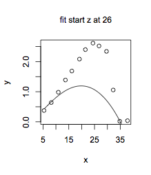
Second, "fitting an equation" generally means having a general form of a relation between $y$ and $x$ in mind, but the details of the form depend on some additional unknown parameters of the equation. "Fitting" then means using the data to estimate the values of the parameters that best match the data, say by minimizing the sum of the squares of the discrepancies between the curve and the data. That is what's implicit in the form of the equation in your comment. (I corrected an apparently missing parenthesis so that it matches your original parameter-free equation at $z=25$):
$$y = \frac{35-x}{35-z}\left(\frac{x}{z}\right)^{(z/10)}$$
Now there is something to "fit": find the value of $z$ that comes closest to your data. The simplest R function to do this is nls. (The R code I used is at the end of the answer.) The best fit to your $x$ and $y$ data is provided by a $z$ value of 33.1, not the value of 25 that would match your first parameter-free equation. It comes closer, but doesn't do very well, either, substantially below most of the true values:
Dangers in fitting equations
Third, you must be very careful if you head down this fitting path. As John von Neumann allegedly said, "With four parameters I can fit an elephant, and with five I can make him wiggle his trunk." Overfitting is a serious temptation when you start playing with data.
FinallyComparing fits to different data sets
If you want to compare the parameter values fitted to two different data sets, it's best to start by examining whether the overall fits differ between the data sets. There is a "useful and rather easily overlooked" way to do this with nls as Peter Dalgaard put it in a recent answer on R-help. (It can be found at the very bottom of the nls help page.)
Instead of working with separate vectors of $x$ and $y$ values from different experiments, construct a pooled data frame containing all the data. Each row should contain an $x$ value, the associated observed $y$ value, and a factor variable indicating the specific experiment. (Make sure the experiments are coded as factors, not as numbers.)
nls then allows you to fit different sets of parameter values to different experiments. Instead of specifying general parameters like Topt in your call, you can subscript the parameters by experiment, e.g. Topt[expt], where "expt" is the name of the factor distinguishing experiments.
Thus you can use anova to compare a fit to all the data, ignoring individual experiments, against a fit that allows different parameter values for different experiments. If these fits aren't statistically distinguishable, then you shouldn't be looking at differences of individual fitted parameter values among experiments. There's an example below where I present R code.
If the fits do differ, then you can consider comparing fitted parameter values. In the limit of very large samples the fitted values should have normal distributions, but it's not clear what "large" means for nonlinear fits and the meaning might differ depending on the equation. Thus there will be questions about the validity of p-values.
If you are willing to assume normality, nls reports standard errors for the parameter values, which you can use to obtain p-values under that assumption. A z-test can provide a rough overview, but it would probably be better to use the approach of Welch's t-test, which allows for different standard errors and degrees of freedom between two parameter estimates. To apply that approach, note that terms like $\frac{s_i^2}{N_i}$ in the formula for Welch's test are equivalent to $SE_i^2$ in the nls output.
R code
In terms of R code, it was simplest to define a general function for your temperature-response curve:
plot(x,y,main="fit z, a, b")
curve(trcFunc(x,33.98,36.74,17.84),add=TRUE)
New form for relation; comparing fits A new general form for the relation of $y$ to $x$ was proposed in an edit to the OP, in which the peak value of $y$ occurs at $x=T_{opt}$. The general form needs an additional parameter to handle the actual peak value of $y$, so I used this modification:
$$y = Y_{max}\frac{T_{max}-x}{T_{max}-T_{opt}}\left(\frac{x}{T_{opt}}\right)^{(T_{opt}/(T_{max}-T_{opt}))}$$
The new general function was defined as:
newFunc <- function(x,Topt,Tmax,Ymax){Ymax*((Tmax-x)/(Tmax-Topt))*(x/Topt)^(Topt/(Tmax-Topt))}
For comparing two experiments, take expt1 as the data in the OP and expt2 as the second data set provided in a comment to this answer, and construct a pooled data frame as suggested above. Then the fit ignoring the differences between experiments is:
fitPool <- nls(y~newFunc(x,Topt,Tmax,Ymax),data=newDF,start=list(Topt=25,Tmax=35,Ymax=2.5))
and that allowing separate parameter values for the two experiments is:
fitSeparate <- nls(y~newFunc(x,Topt[expt],Tmax[expt],Ymax[expt]),data=newDF,start=list(Topt=c(25,25),Tmax=c(35,35),Ymax=c(2.5,2.5)))
The pooled and separate fits are not significantly different:
> anova(fitPool,fitSeparate)
Analysis of Variance Table
Model 1: y ~ newFunc(x, Topt, Tmax, Ymax)
Model 2: y ~ newFunc(x, Topt[expt], Tmax[expt], Ymax[expt])
  Res.Df Res.Sum Sq Df  Sum Sq F value Pr(>F)
1     19     1.9215
2     16     1.4410  3 0.48046  1.7782 0.1918
Warning on choice of starting values

