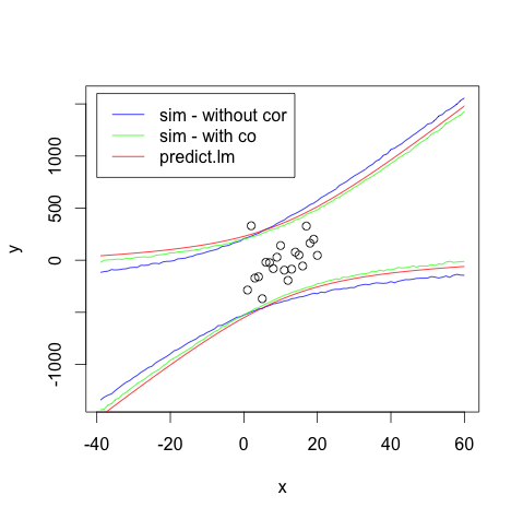
Thanks to atireto's comment, I realized that I haven't taken into account the covariances between the estimated parameters. I was assuming that a and b are uncorrelated random variables, but they are not. So I corrected the sampling of a and b by converting them to correlated random variables using Cholesky decomposition of variance-covariance matrix (see here).

Here's the corrected code:

rm(list = ls())

n = 20     # number of points
N = 10000  # simulation rounds
x = 1:n    # x
s = 200    # standard deviation of error

set.seed(12)
e = rnorm(n, 0, s)

a = 5; b = 5  # slope, intercept

y = a * x + b + e

## lm model
mod1 = lm(y ~ x)
summ_mod1 = summary(mod1)

## std errors
coefs = summ_mod1$coefficients[, 1:2]
sigma = summ_mod1$sigma

## predict new data using simulation
new.x = (min(x) - 2 * max(x)):(max(x) + 2 * max(x))

upper = rep(0, length(new.x))
lower = rep(0, length(new.x))
tmp   = rep(0, N)

for (i in 1:length(new.x)) {
  tmp = rnorm(n = N, mean = coefs[1, 1], sd = coefs[1, 2]) +
        rnorm(n = N, mean = coefs[2, 1], sd = coefs[2, 2]) * new.x[i] +
        rnorm(n = N, mean = 0, sd = sigma)
  
  upper[i] = mean(tmp) + 1.96 * sd(tmp)
  lower[i] = mean(tmp) - 1.96 * sd(tmp)
}

plot(x, y, type = "p", 
     xlim = c(min(new.x), max(new.x)),
     ylim = c(min(lower), max(upper)))
lines(new.x, lower, col = "blue")
lines(new.x, upper, col = "blue")

## R's prediction interval
pred.int =  predict(object = mod1, 
                    newdata = data.frame(x = new.x), 
                    interval = "predict",
                    level = 0.95)

pred.lower = pred.int[,2]
pred.upper = pred.int[,3]

lines(new.x, pred.lower, col = "red")
lines(new.x, pred.upper, col = "red")

## taking the variance-covariance matrix into account
L = chol(vcov(mod1))

for (i in 1:length(new.x)) {
  beta = matrix(c(rnorm(n = N),
                  rnorm(n = N)), 
                nrow = 2)
  
  beta_cor = t(L) %*% beta
  
  tmp = coefs[1, 1] + beta_cor[1, ] +
        (coefs[2, 1] + beta_cor[2, ]) * new.x[i] +
        rnorm(n = N, mean = 0, sd = sigma)
  
  upper[i] = mean(tmp) + 1.96 * sd(tmp)
  lower[i] = mean(tmp) - 1.96 * sd(tmp)
}

lines(new.x, lower, col = "green")
lines(new.x, upper, col = "green")

legend(x = -40, y = 1600, 
       legend = c("sim - without cor", "sim - with co", "predict.lm"),
       lty = c(1, 1, 1),
       col = c("blue", "green", "red"))

It still doesn't perfectly match the R's predict.lm result, but it's very close. In fact, if I change the 1.96 coefficient to something like 2.1, it matches it perfectly. Predict.lm is supposed to be 95% prediction interval, so I'm not sure this is happening.