R added
Source Link
luchonacho
  • 2.7k
  • 5
  • 26
  • 47

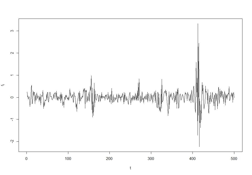
In finance, GARCH (generalized autoregressive conditional heteroskedasticity) effects are widely cited here: stock returns $r_t:=(P_t-P_{t-1})/P_{t-1}$, with $P_t$ the price at time $t$, themselves are uncorrelated with their own past $r_{t-1}$ if stock markets are efficient (else, you could easily and profitably predict where prices are going), but their squares $r_t^2$ and $r_{t-1}^2$ are not: there is time dependence in the variances, which cluster in time, with periods of high variance in volatile times.

Here is an artificial example (yet again, I know, but "real" stock return series may well look similar):

enter image description here

You see the high volatility cluster around in particular $t\approx400$.

Generated using R code:

library(TSA)
garch01.sim <- garch.sim(alpha=c(.01,.55),beta=0.4,n=500)
plot(garch01.sim, type='l', ylab=expression(r[t]),xlab='t')

In finance, GARCH (generalized autoregressive conditional heteroskedasticity) effects are widely cited here: stock returns $r_t:=(P_t-P_{t-1})/P_{t-1}$, with $P_t$ the price at time $t$, themselves are uncorrelated with their own past $r_{t-1}$ if stock markets are efficient (else, you could easily and profitably predict where prices are going), but their squares $r_t^2$ and $r_{t-1}^2$ are not: there is time dependence in the variances, which cluster in time, with periods of high variance in volatile times.

Here is an artificial example (yet again, I know, but "real" stock return series may well look similar):

enter image description here

You see the high volatility cluster around in particular $t\approx400$.

Generated using

library(TSA)
garch01.sim <- garch.sim(alpha=c(.01,.55),beta=0.4,n=500)
plot(garch01.sim, type='l', ylab=expression(r[t]),xlab='t')

In finance, GARCH (generalized autoregressive conditional heteroskedasticity) effects are widely cited here: stock returns $r_t:=(P_t-P_{t-1})/P_{t-1}$, with $P_t$ the price at time $t$, themselves are uncorrelated with their own past $r_{t-1}$ if stock markets are efficient (else, you could easily and profitably predict where prices are going), but their squares $r_t^2$ and $r_{t-1}^2$ are not: there is time dependence in the variances, which cluster in time, with periods of high variance in volatile times.

Here is an artificial example (yet again, I know, but "real" stock return series may well look similar):

enter image description here

You see the high volatility cluster around in particular $t\approx400$.

Generated using R code:

library(TSA)
garch01.sim <- garch.sim(alpha=c(.01,.55),beta=0.4,n=500)
plot(garch01.sim, type='l', ylab=expression(r[t]),xlab='t')
added 98 characters in body
Source Link
Christoph Hanck
  • 34.8k
  • 3
  • 78
  • 137

In finance, GARCH (generalized autoregressive conditional heteroskedasticity) effects are widely cited here: stock returns $r_t:=(P_t-P_{t-1})/P_{t-1}$, with $P_t$ the price at time $t$, themselves are uncorrelated with their own past $r_{t-1}$ if stock markets are efficient (else, you could easily and profitably predict where prices are going), but their squares $r_t^2$ and $r_{t-1}^2$ are not: there is time dependence in the variances, which cluster in time, with periods of high variance in volatile times.

Here is an artificial example (yet again, I know, but "real" stock return series may well look similar):

enter image description here

You see the high volatility cluster around in particular $t\approx400$.

Generated using

library(TSA)
garch01.sim <- garch.sim(alpha=c(.01,.55),beta=0.4,n=500)
plot(garch01.sim, type='l', ylab=expression(r[t]),xlab='t')

In finance, GARCH (generalized autoregressive conditional heteroskedasticity) effects are widely cited here: stock returns themselves are uncorrelated with their own past if stock markets are efficient (else, you could easily and profitably predict where prices are going), but their squares are not: there is time dependence in the variances, which cluster in time, with periods of high variance in volatile times.

Here is an artificial example (yet again, I know, but "real" stock return series may well look similar):

enter image description here

You see the high volatility cluster around in particular $t\approx400$.

Generated using

library(TSA)
garch01.sim <- garch.sim(alpha=c(.01,.55),beta=0.4,n=500)
plot(garch01.sim, type='l', ylab=expression(r[t]),xlab='t')

In finance, GARCH (generalized autoregressive conditional heteroskedasticity) effects are widely cited here: stock returns $r_t:=(P_t-P_{t-1})/P_{t-1}$, with $P_t$ the price at time $t$, themselves are uncorrelated with their own past $r_{t-1}$ if stock markets are efficient (else, you could easily and profitably predict where prices are going), but their squares $r_t^2$ and $r_{t-1}^2$ are not: there is time dependence in the variances, which cluster in time, with periods of high variance in volatile times.

Here is an artificial example (yet again, I know, but "real" stock return series may well look similar):

enter image description here

You see the high volatility cluster around in particular $t\approx400$.

Generated using

library(TSA)
garch01.sim <- garch.sim(alpha=c(.01,.55),beta=0.4,n=500)
plot(garch01.sim, type='l', ylab=expression(r[t]),xlab='t')
added 668 characters in body
Source Link
Christoph Hanck
  • 34.8k
  • 3
  • 78
  • 137

In finance, ARCHGARCH (generalized autoregressive conditional heteroskedasticity) effects are widely cited here: stock returns themselves are uncorrelated with their own past if stock markets are efficient (else, you could easily and profitably predict where prices are going), but their squares are not, as: there is time dependence in the variances, which cluster in time, with periods of high variance in volatile times.

Here is an artificial example (yet again, I know, but "real" stock return series may well look similar):

enter image description here

You see the high volatility cluster around in particular $t\approx400$.

Generated using

library(TSA)
garch01.sim <- garch.sim(alpha=c(.01,.55),beta=0.4,n=500)
plot(garch01.sim, type='l', ylab=expression(r[t]),xlab='t')

In finance, ARCH effects are widely cited here: stock returns themselves are uncorrelated if stock markets are efficient, but their squares are not, as there is time dependence in the variances, which cluster in time, with periods of high variance in volatile times.

In finance, GARCH (generalized autoregressive conditional heteroskedasticity) effects are widely cited here: stock returns themselves are uncorrelated with their own past if stock markets are efficient (else, you could easily and profitably predict where prices are going), but their squares are not: there is time dependence in the variances, which cluster in time, with periods of high variance in volatile times.

Here is an artificial example (yet again, I know, but "real" stock return series may well look similar):

enter image description here

You see the high volatility cluster around in particular $t\approx400$.

Generated using

library(TSA)
garch01.sim <- garch.sim(alpha=c(.01,.55),beta=0.4,n=500)
plot(garch01.sim, type='l', ylab=expression(r[t]),xlab='t')
Source Link
Christoph Hanck
  • 34.8k
  • 3
  • 78
  • 137
Loading