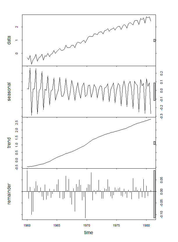
UPDATE :

So, I tried a few different things and this is what I learnt:

a) In order to fit the trend, I can first extract the trend time series generated by the stl() function in R and then perform fitting on it as follows:

     > Trend=decomp_JJ$time.series[,2] 
     > t=time(decomp_JJ$time.series[,2])
     > fit_Trend=lm(Trend~0+t)
     > summary(fit_Trend)
        Call:
       lm(formula = Trend ~ 0 + t)

       Residuals:
            Min       1Q   Median       3Q      Max 
         -1.55503 -0.90810  0.07018  0.87686  1.60349 

       Coefficients:
          Estimate Std. Error t value Pr(>|t|)    
        t 5.628e-04  5.648e-05   9.965 7.72e-16 ***
        ---
        Signif. codes:  0 ‘***’ 0.001 ‘**’ 0.01 ‘*’ 0.05 ‘.’ 0.1 ‘ ’ 1

         Residual standard error: 1.02 on 83 degrees of freedom
         Multiple R-squared:  0.5447,   Adjusted R-squared:  0.5392 
         F-statistic:  99.3 on 1 and 83 DF,  p-value: 7.723e-16

but I am not sure, if this is the correct way to proceed. Also, I haven't still figured out how to fit the seasonal component

I am very new to Time Series Analysis (together with R). I have been practising with some very simple datasets to understand how to decompose the time series into Trend, Seasonal and Error components and then check whether the Error component is Gaussian or not. Till this point, everything is pretty much clear to me. However, after the decomposition, how do I fit the trend and seasonal component (using R)? I am confused on 'to what' do I fit my trend and seasonal component? I mean what should my predictors be? For the trend, I can use the time (specifically for the example below, the four quarters) perhaps? And as such, what does the fitting of seasonal component imply and how can it be achieved?

Below is one of time series datasets that I used. This time series is called 'jj' and is present in the 'astsa' package. The frequency of this time series is quarterly.:

    > jj
         Qtr1      Qtr2      Qtr3      Qtr4
  1960  0.710000  0.630000  0.850000  0.440000
  1961  0.610000  0.690000  0.920000  0.550000
  1962  0.720000  0.770000  0.920000  0.600000
  1963  0.830000  0.800000  1.000000  0.770000
  1964  0.920000  1.000000  1.240000  1.000000
  1965  1.160000  1.300000  1.450000  1.250000
  1966  1.260000  1.380000  1.860000  1.560000
  1967  1.530000  1.590000  1.830000  1.860000
  1968  1.530000  2.070000  2.340000  2.250000
  1969  2.160000  2.430000  2.700000  2.250000
  1970  2.790000  3.420000  3.690000  3.600000
  1971  3.600000  4.320000  4.320000  4.050000
  1972  4.860000  5.040000  5.040000  4.410000
  1973  5.580000  5.850000  6.570000  5.310000
  1974  6.030000  6.390000  6.930000  5.850000
  1975  6.930000  7.740000  7.830000  6.120000
  1976  7.740000  8.910000  8.280000  6.840000
  1977  9.540000 10.260000  9.540000  8.729999
  1978 11.880000 12.060000 12.150000  8.910000
  1979 14.040000 12.960000 14.850000  9.990000
  1980 16.200000 14.670000 16.020000 11.610000

    > decomp_JJ=stl(log(jj),s.window = 4)
    > plot(decomp_JJ)

Any help on this is much appreciated!

I am very new to Time Series Analysis (together with R). I have been practising with some very simple datasets to understand how to decompose the time series into Trend, Seasonal and Error components and then check whether the Error component is Gaussian or not. Till this point, everything is pretty much clear to me. However, after the decomposition, how do I fit the trend and seasonal component (using R)? I am confused on 'to what' do I fit my trend and seasonal component? I mean what should my predictors be? For the trend, I can use the time (specifically for the example below, the four quarters) perhaps? And as such, what does the fitting of seasonal component imply and how can it be achieved?

Below is one of time series datasets that I used. This time series is called jj and is present in the astsa package. The frequency of this time series is quarterly.:

    > jj
         Qtr1      Qtr2      Qtr3      Qtr4
  1960  0.710000  0.630000  0.850000  0.440000
  1961  0.610000  0.690000  0.920000  0.550000
  1962  0.720000  0.770000  0.920000  0.600000
  1963  0.830000  0.800000  1.000000  0.770000
  1964  0.920000  1.000000  1.240000  1.000000
  1965  1.160000  1.300000  1.450000  1.250000
  1966  1.260000  1.380000  1.860000  1.560000
  1967  1.530000  1.590000  1.830000  1.860000
  1968  1.530000  2.070000  2.340000  2.250000
  1969  2.160000  2.430000  2.700000  2.250000
  1970  2.790000  3.420000  3.690000  3.600000
  1971  3.600000  4.320000  4.320000  4.050000
  1972  4.860000  5.040000  5.040000  4.410000
  1973  5.580000  5.850000  6.570000  5.310000
  1974  6.030000  6.390000  6.930000  5.850000
  1975  6.930000  7.740000  7.830000  6.120000
  1976  7.740000  8.910000  8.280000  6.840000
  1977  9.540000 10.260000  9.540000  8.729999
  1978 11.880000 12.060000 12.150000  8.910000
  1979 14.040000 12.960000 14.850000  9.990000
  1980 16.200000 14.670000 16.020000 11.610000

    > decomp_JJ=stl(log(jj),s.window = 4)
    > plot(decomp_JJ)

Any help on this is much appreciated!