I've recently run into a situation where I know a few probability points in the tail of a distribution and I want to "fit" a distribution that goes through these points in the tail. I realize this is messy and not overly accurate, and plagued with conceptual issues. However, trust me that I really want to do this.
So effectively I know some points in the tail of the CDF with x being the values and y being the probability of that value or smaller. Here's R code to illustrate my data:
x <- c(0.55, 0.6, 0.65, 0.7, 0.75, 0.8, 0.85)
y <- c(0.0666666666666667, 0.0625, 0.0659340659340659, 0.0563106796116505,
0.0305676855895196, 0.0436953807740325, 0.0267459138187221)
Then I create a function to minimize error between my data and a beta distribution CDF using pbeta. I use SSE as a fit metric then minimize that with -sum
# function to optomize with optim
beta_func <- function(par, x) -sum( (pbeta( x, par[1], par[2]) - y)**2 )
out <- optim(c(1,.2), beta_func, lower=c(9,.8), upper=c(200,200), method="L-BFGS-B", x=x)
out <- out$par
print(out)
#> [1]  0.90000 23.40294
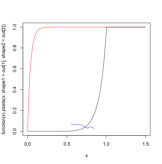
Below I graph the 'optimized' beta distribution in red, my actual data in blue, and a hand tweaked starting guess of the beta parameters in black.
plot(function(x) pbeta(x, shape1=out[1], shape2=out[2] ), 0, 1.5, col='red')
plot(function(x) pbeta(x, 9,.8), 0, 1.5, col='black', add=TRUE)
lines(x,y, col='blue')

I can't grok what's going on with optim to give a solution that's worse than my starting guess. I went in manually calculated the SSE for my starting guess vs the optim solution and it looks like my guess has a much larger -SSE:
# my guess
-sum( (pbeta( x, 9, .8) - y)**2)
#> [1] -0.03493344

# optim's output
-sum( (pbeta( x, .9, 23) - y)**2)
#> [1] -6.314587
Using past history as my Bayesian prior, my guess is that I'm misunderstanding optim or feeding it improper inputs. However I can't grok what's going on. Any tips would be greatly appreciated.

