added 129 characters in body
Source Link
IrishStat
  • 30k
  • 5
  • 36
  • 60

you said:

Make product demand series and indicator candidate series stationary (for example through differencing)

I say : Not necessarily as you my be vitiating the importance of the predictor series by pre-empting the effect

Iteratively compare the product demand series with the indicator candidate series' using cross-correlation - looking for leads, lags and contemporaneous effects with high correlation and picking indicators with high cross-correlation using pre-whitening procedures as discussed here Why is prewhitening important? and here The theory behind fitting an ARIMAX model

Post an example of one of your favorite products and I will try and help further .

P.S. in the absence of the causal series your Y series seems to have a level/step change at the last 16 or so observations. Note that a level/step change is in reality an INTERCEPT CHANGE . When you introduce your X predictor it's downwards activity for the latter part of the series might "explain" the level/step shift in Y .

EDITED AFTER RECEIPT OF DATA:

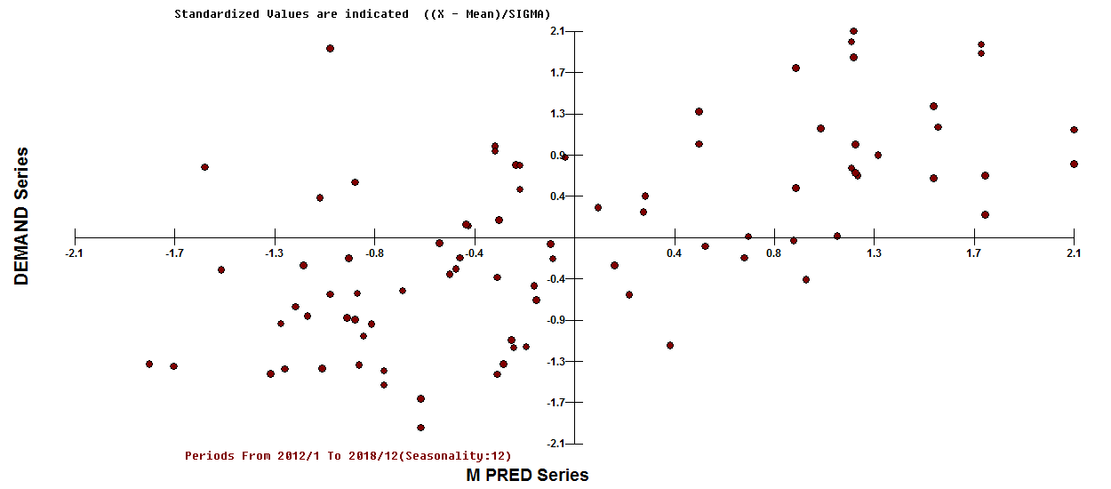
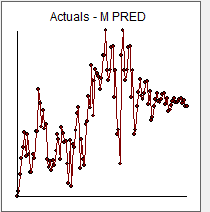
The PRED series that you posted is different from the one you originally included, I detected a zero in it and I remedied it and used it as a candidate to predict Y DEMAND) Here is a plot of PRED enter image description here and a scaled plot of DEMAND vs PRED enter image description here visually suggesting some outside effects , possibly repetitious ...possibly permanent ,,,possibly 1 time only AND a general positive relationship i.e.an upwards trend between SCALED DEMAND and SCALED PRED.
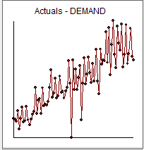
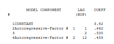
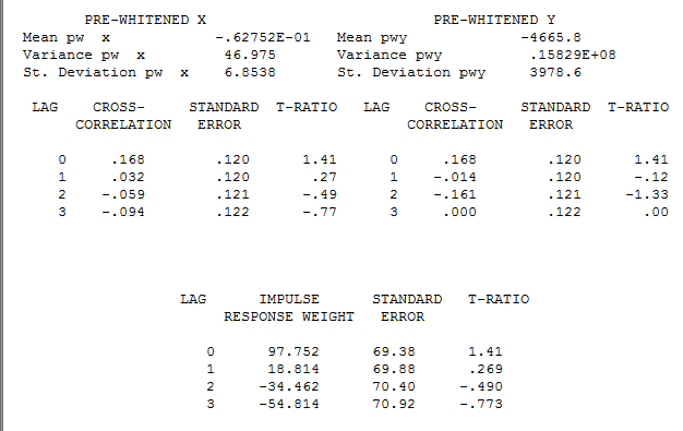
The pre-whitening model for X is here enter image description here suggesting an expanded filter containing 15 coefficients , 10 of which are zero.
The pre-whitened cross-correlation is here suggesting a contemporaneous effect

enter image description here

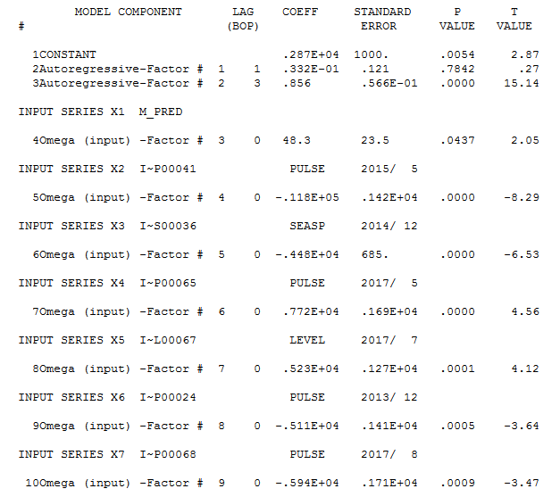
Intervention Detection suggested adding s few predictors reflecting the "omitted structure" . Here is the equation enter image description here with more detail here enter image description here. The repetitive effects are a negative seasonal pulse for December and a positive level shift starting at July of 2017 ( 17 PERIODS AGO confirming a prior visual finding made before the actual data was received and analyzed) . The non-repetitive anomalies are nearly all visually obvious .

The statistics for this model are here enter image description here
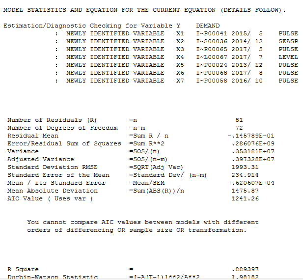
The unusual points were 5 in number reflecting one time anomalies.

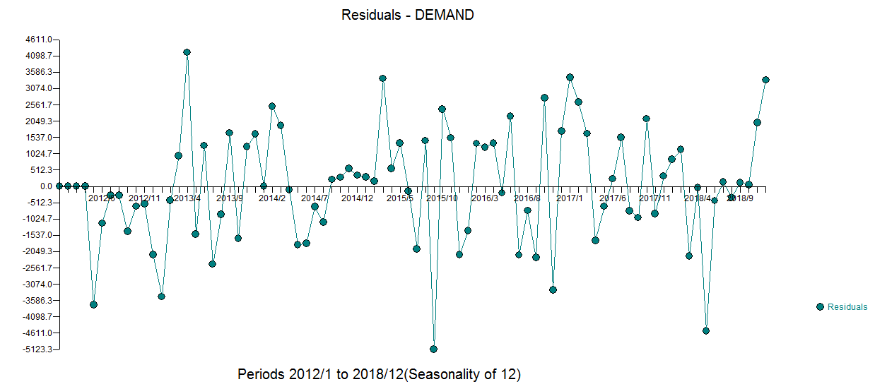
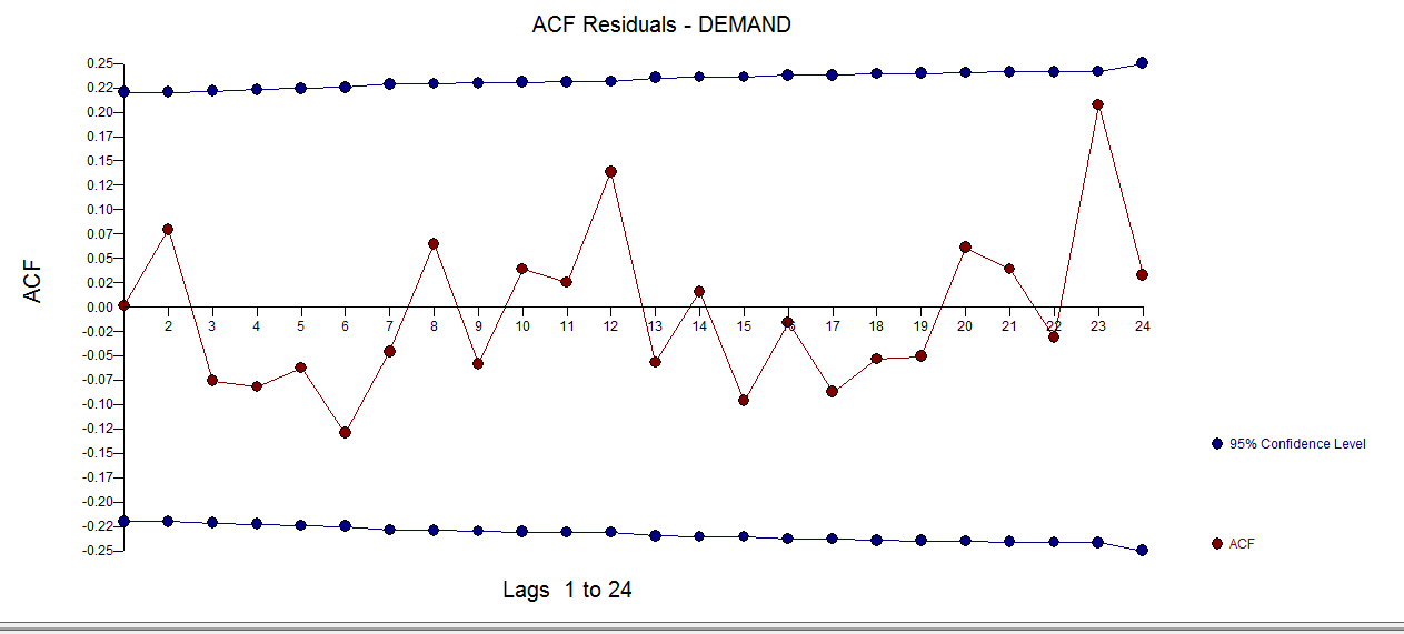
Following is the Actual,Fit and Forecast graph enter image description here with residual plot here enter image description here and acf here enter image description here
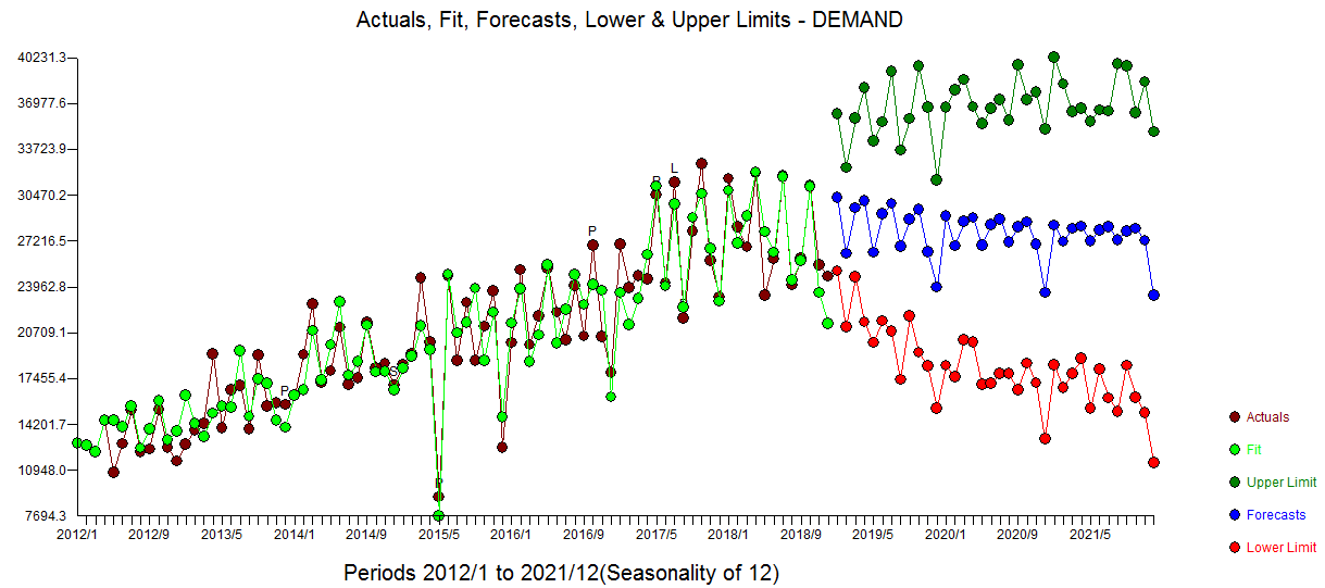
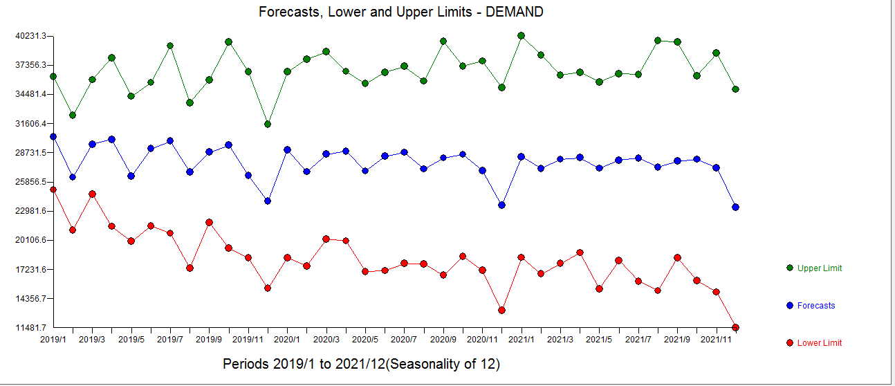
Finally the Forecast plot is here based upon forecasts generated for the predictor series PRED enter image description here . The confidence intervals include the uncertainty in the predicted PRED and the possibility that future anomalies will be encountered.
In summary there is no need to difference the data in order to build a possibly useful model.

I used an (optionally automated) piece of software [AUTOBOX] that I have helped to develop. This is not meant as an advertisement but as a disclaimer.

Be very aware of the complicated ARIMA portion that was detected reflecting a typical STRONG QUARTERLY EFFECT typical in national account series. Kudos to @chrishmorris for his acumen/eyesight for visually detecting the strong quarterly effect for this monthly series AND SUGGESTING A 3 PERIOD AVERAGE be employed. Note that the value 3 periods ago is optimally weighted by .856 . The final model includes a 3 period weighted average with values .033 for lag 1 , 0. for lag 2 and .856 for lag 3 .

Finally if the OP wishes to specify future values for PRED these are easily used to create alternative forecasts for DEMAND . We show here the 84 historical values for PRED with ARIMA predictions for the next 36 periods. enter image description here
you said:

Make product demand series and indicator candidate series stationary (for example through differencing)

I say : Not necessarily as you my be vitiating the importance of the predictor series by pre-empting the effect

Iteratively compare the product demand series with the indicator candidate series' using cross-correlation - looking for leads, lags and contemporaneous effects with high correlation and picking indicators with high cross-correlation using pre-whitening procedures as discussed here Why is prewhitening important? and here The theory behind fitting an ARIMAX model

Post an example of one of your favorite products and I will try and help further .

P.S. in the absence of the causal series your Y series seems to have a level/step change at the last 16 or so observations. Note that a level/step change is in reality an INTERCEPT CHANGE . When you introduce your X predictor it's downwards activity for the latter part of the series might "explain" the level/step shift in Y .

EDITED AFTER RECEIPT OF DATA:

The PRED series that you posted is different from the one you originally included, I detected a zero in it and I remedied it and used it as a candidate to predict Y DEMAND) Here is a plot of PRED enter image description here and a scaled plot of DEMAND vs PRED enter image description here visually suggesting some outside effects , possibly repetitious ...possibly permanent ,,,possibly 1 time only AND a general positive relationship i.e.an upwards trend between SCALED DEMAND and SCALED PRED.

The pre-whitening model for X is here enter image description here suggesting an expanded filter containing 15 coefficients , 10 of which are zero.

The pre-whitened cross-correlation is here suggesting a contemporaneous effect

enter image description here

Intervention Detection suggested adding s few predictors reflecting the "omitted structure" . Here is the equation enter image description here with more detail here enter image description here. The repetitive effects are a negative seasonal pulse for December and a positive level shift starting at July of 2017 ( 17 PERIODS AGO confirming a prior visual finding made before the actual data was received and analyzed) . The non-repetitive anomalies are nearly all visually obvious .

The unusual points were 5 in number reflecting one time anomalies.

Following is the Actual,Fit and Forecast graph enter image description here with residual plot here enter image description here and acf here enter image description here

Finally the Forecast plot is here based upon forecasts generated for the predictor series PRED enter image description here . The confidence intervals include the uncertainty in the predicted PRED and the possibility that future anomalies will be encountered.

In summary there is no need to difference the data in order to build a possibly useful model.

I used an (optionally automated) piece of software [AUTOBOX] that I have helped to develop. This is not meant as an advertisement but as a disclaimer.

Be very aware of the complicated ARIMA portion that was detected reflecting a typical STRONG QUARTERLY EFFECT typical in national account series. Kudos to @chrishmorris for his acumen/eyesight for visually detecting the strong quarterly effect for this monthly series AND SUGGESTING A 3 PERIOD AVERAGE be employed. Note that the value 3 periods ago is optimally weighted by .856 . The final model includes a 3 period weighted average with values .033 for lag 1 , 0. for lag 2 and .856 for lag 3 .

Finally if the OP wishes to specify future values for PRED these are easily used to create alternative forecasts for DEMAND . We show here the 84 historical values for PRED with ARIMA predictions for the next 36 periods. enter image description here

you said:

Make product demand series and indicator candidate series stationary (for example through differencing)

I say : Not necessarily as you my be vitiating the importance of the predictor series by pre-empting the effect

Iteratively compare the product demand series with the indicator candidate series' using cross-correlation - looking for leads, lags and contemporaneous effects with high correlation and picking indicators with high cross-correlation using pre-whitening procedures as discussed here Why is prewhitening important? and here The theory behind fitting an ARIMAX model

Post an example of one of your favorite products and I will try and help further .

P.S. in the absence of the causal series your Y series seems to have a level/step change at the last 16 or so observations. Note that a level/step change is in reality an INTERCEPT CHANGE . When you introduce your X predictor it's downwards activity for the latter part of the series might "explain" the level/step shift in Y .

EDITED AFTER RECEIPT OF DATA:

The PRED series that you posted is different from the one you originally included, I detected a zero in it and I remedied it and used it as a candidate to predict Y DEMAND) Here is a plot of PRED enter image description here and a scaled plot of DEMAND vs PRED enter image description here visually suggesting some outside effects , possibly repetitious ...possibly permanent ,,,possibly 1 time only AND a general positive relationship i.e.an upwards trend between SCALED DEMAND and SCALED PRED.

The pre-whitening model for X is here enter image description here suggesting an expanded filter containing 15 coefficients , 10 of which are zero.

The pre-whitened cross-correlation is here suggesting a contemporaneous effect

enter image description here

Intervention Detection suggested adding s few predictors reflecting the "omitted structure" . Here is the equation enter image description here with more detail here enter image description here. The repetitive effects are a negative seasonal pulse for December and a positive level shift starting at July of 2017 ( 17 PERIODS AGO confirming a prior visual finding made before the actual data was received and analyzed) . The non-repetitive anomalies are nearly all visually obvious .

The statistics for this model are here enter image description here

The unusual points were 5 in number reflecting one time anomalies.

Following is the Actual,Fit and Forecast graph enter image description here with residual plot here enter image description here and acf here enter image description here

Finally the Forecast plot is here based upon forecasts generated for the predictor series PRED enter image description here . The confidence intervals include the uncertainty in the predicted PRED and the possibility that future anomalies will be encountered.

In summary there is no need to difference the data in order to build a possibly useful model.

I used an (optionally automated) piece of software [AUTOBOX] that I have helped to develop. This is not meant as an advertisement but as a disclaimer.

Be very aware of the complicated ARIMA portion that was detected reflecting a typical STRONG QUARTERLY EFFECT typical in national account series. Kudos to @chrishmorris for his acumen/eyesight for visually detecting the strong quarterly effect for this monthly series AND SUGGESTING A 3 PERIOD AVERAGE be employed. Note that the value 3 periods ago is optimally weighted by .856 . The final model includes a 3 period weighted average with values .033 for lag 1 , 0. for lag 2 and .856 for lag 3 .

Finally if the OP wishes to specify future values for PRED these are easily used to create alternative forecasts for DEMAND . We show here the 84 historical values for PRED with ARIMA predictions for the next 36 periods. enter image description here
added 29 characters in body
Source Link
IrishStat
  • 30k
  • 5
  • 36
  • 60

you said:

Make product demand series and indicator candidate series stationary (for example through differencing)

I say : Not necessarily as you my be vitiating the importance of the predictor series by pre-empting the effect

Iteratively compare the product demand series with the indicator candidate series' using cross-correlation - looking for leads, lags and contemporaneous effects with high correlation and picking indicators with high cross-correlation using pre-whitening procedures as discussed here Why is prewhitening important? and here The theory behind fitting an ARIMAX model

Post an example of one of your favorite products and I will try and help further .

P.S. in the absence of the causal series your Y series seems to have a level/step change at the last 16 or so observations. Note that a level/step change is in reality an INTERCEPT CHANGE . When you introduce your X predictor it's downwards activity for the latter part of the series might "explain" the level/step shift in Y .

EDITED AFTER RECEIPT OF DATA:

The PRED series that you posted is different from the one you originally included, I detected a zero in it and I remedied it and used it as a candidate to predict Y DEMAND) Here is a plot of PRED enter image description here and a scaled plot of DEMAND vs PRED enter image description here visually suggesting some outside effects , possibly repetitious ...possibly permanent ,,,possibly 1 time only AND a general positive relationship i.e.an upwards trend between SCALED DEMAND and SCALED PRED.

The pre-whitening model for X is here enter image description here suggesting an expanded filter containing 15 coefficients , 10 of which are zero.

The pre-whitened cross-correlation is here suggesting a contemporaneous effect

enter image description here

Intervention Detection suggested adding s few predictors reflecting the "omitted structure" . Here is the equation enter image description here with more detail here enter image description here. The repetitive effects are a negative seasonal pulse for December and a positive level shift starting at July of 2017 ( 17 PERIODS AGO confirming a prior visual finding made before the actual data was received and analyzed) . The non-repetitive anomalies are nearly all visually obvious .

The unusual points were 5 in number reflecting one time anomalies.

Following is the Actual,Fit and Forecast graph enter image description here with residual plot here enter image description here and acf here enter image description here

Finally the Forecast plot is here based upon forecasts generated for the predictor series PRED enter image description here . The confidence intervals include the uncertainty in the predicted PRED and the possibility that future anomalies will be encountered.

In summary there is no need to difference the data in order to build a possibly useful model.

I used an (optionally automated) piece of software [AUTOBOX] that I have helped to develop. This is not meant as an advertisement but as a disclaimer.

Be very areaware of the complicated ARIMA portion that was detected reflecting a typical STRONG QUARTERLY EFFECT typical in nationalllynational account series. Kudos to @chrishmorris for his acumen in/eyesight for visually detecting thisthe strong quarterly effect for athis monthly series AND SUGGESTING A 3 PERIOD AVERAGE be employed. Note that the value 3 periods ago is optimally weighted by .856 .. essentiallyThe final model includes a 3 period weighted average with values .033 for lag 1 , 0. for lag 2 and .856 for lag 3 .

Finally if the OP wishes to specify future values for PRED these are easily used to create alternative forecasts for DEMAND . We show here the 84 historical values for PRED and thewith ARIMA predictions frofor the next 36 periods. enter image description here

you said:

Make product demand series and indicator candidate series stationary (for example through differencing)

I say : Not necessarily as you my be vitiating the importance of the predictor series by pre-empting the effect

Iteratively compare the product demand series with the indicator candidate series' using cross-correlation - looking for leads, lags and contemporaneous effects with high correlation and picking indicators with high cross-correlation using pre-whitening procedures as discussed here Why is prewhitening important? and here The theory behind fitting an ARIMAX model

Post an example of one of your favorite products and I will try and help further .

P.S. in the absence of the causal series your Y series seems to have a level/step change at the last 16 or so observations. Note that a level/step change is in reality an INTERCEPT CHANGE . When you introduce your X predictor it's downwards activity for the latter part of the series might "explain" the level/step shift in Y .

EDITED AFTER RECEIPT OF DATA:

The PRED series that you posted is different from the one you originally included, I detected a zero in it and I remedied it and used it as a candidate to predict Y DEMAND) Here is a plot of PRED enter image description here and a scaled plot of DEMAND vs PRED enter image description here visually suggesting some outside effects , possibly repetitious ...possibly permanent ,,,possibly 1 time only AND a general positive relationship i.e.an upwards trend between SCALED DEMAND and SCALED PRED.

The pre-whitening model for X is here enter image description here suggesting an expanded filter containing 15 coefficients , 10 of which are zero.

The pre-whitened cross-correlation is here suggesting a contemporaneous effect

enter image description here

Intervention Detection suggested adding s few predictors reflecting the "omitted structure" . Here is the equation enter image description here with more detail here enter image description here. The repetitive effects are a negative seasonal pulse for December and a positive level shift starting at July of 2017 ( 17 PERIODS AGO confirming a prior visual finding made before the actual data was received and analyzed) . The non-repetitive anomalies are nearly all visually obvious .

The unusual points were 5 in number reflecting one time anomalies.

Following is the Actual,Fit and Forecast graph enter image description here with residual plot here enter image description here and acf here enter image description here

Finally the Forecast plot is here based upon forecasts generated for the predictor series PRED enter image description here . The confidence intervals include the uncertainty in the predicted PRED and the possibility that future anomalies will be encountered.

In summary there is no need to difference the data in order to build a possibly useful model.

I used an (optionally automated) piece of software [AUTOBOX] that I have helped to develop. This is not meant as an advertisement but as a disclaimer.

Be very are of the complicated ARIMA portion that was detected reflecting a typical STRONG QUARTERLY EFFECT in nationallly account series. Kudos to @chrishmorris for his acumen in visually detecting this strong quarterly effect for a monthly series AND SUGGESTING A 3 PERIOD AVERAGE be employed. Note that the value 3 periods ago is optimally weighted by .856 .. essentially a 3 period weighted average with values .033 for lag 1 , 0. for lag 2 and .856 for lag 3

Finally if the OP wishes to specify future values for PRED these are easily used to create alternative forecasts for DEMAND . We show here the 84 historical values for PRED and the ARIMA predictions fro the next 36 periods. enter image description here

you said:

Make product demand series and indicator candidate series stationary (for example through differencing)

I say : Not necessarily as you my be vitiating the importance of the predictor series by pre-empting the effect

Iteratively compare the product demand series with the indicator candidate series' using cross-correlation - looking for leads, lags and contemporaneous effects with high correlation and picking indicators with high cross-correlation using pre-whitening procedures as discussed here Why is prewhitening important? and here The theory behind fitting an ARIMAX model

Post an example of one of your favorite products and I will try and help further .

P.S. in the absence of the causal series your Y series seems to have a level/step change at the last 16 or so observations. Note that a level/step change is in reality an INTERCEPT CHANGE . When you introduce your X predictor it's downwards activity for the latter part of the series might "explain" the level/step shift in Y .

EDITED AFTER RECEIPT OF DATA:

The PRED series that you posted is different from the one you originally included, I detected a zero in it and I remedied it and used it as a candidate to predict Y DEMAND) Here is a plot of PRED enter image description here and a scaled plot of DEMAND vs PRED enter image description here visually suggesting some outside effects , possibly repetitious ...possibly permanent ,,,possibly 1 time only AND a general positive relationship i.e.an upwards trend between SCALED DEMAND and SCALED PRED.

The pre-whitening model for X is here enter image description here suggesting an expanded filter containing 15 coefficients , 10 of which are zero.

The pre-whitened cross-correlation is here suggesting a contemporaneous effect

enter image description here

Intervention Detection suggested adding s few predictors reflecting the "omitted structure" . Here is the equation enter image description here with more detail here enter image description here. The repetitive effects are a negative seasonal pulse for December and a positive level shift starting at July of 2017 ( 17 PERIODS AGO confirming a prior visual finding made before the actual data was received and analyzed) . The non-repetitive anomalies are nearly all visually obvious .

The unusual points were 5 in number reflecting one time anomalies.

Following is the Actual,Fit and Forecast graph enter image description here with residual plot here enter image description here and acf here enter image description here

Finally the Forecast plot is here based upon forecasts generated for the predictor series PRED enter image description here . The confidence intervals include the uncertainty in the predicted PRED and the possibility that future anomalies will be encountered.

In summary there is no need to difference the data in order to build a possibly useful model.

I used an (optionally automated) piece of software [AUTOBOX] that I have helped to develop. This is not meant as an advertisement but as a disclaimer.

Be very aware of the complicated ARIMA portion that was detected reflecting a typical STRONG QUARTERLY EFFECT typical in national account series. Kudos to @chrishmorris for his acumen/eyesight for visually detecting the strong quarterly effect for this monthly series AND SUGGESTING A 3 PERIOD AVERAGE be employed. Note that the value 3 periods ago is optimally weighted by .856 . The final model includes a 3 period weighted average with values .033 for lag 1 , 0. for lag 2 and .856 for lag 3 .

Finally if the OP wishes to specify future values for PRED these are easily used to create alternative forecasts for DEMAND . We show here the 84 historical values for PRED with ARIMA predictions for the next 36 periods. enter image description here

added 270 characters in body
Source Link
IrishStat
  • 30k
  • 5
  • 36
  • 60

you said:

Make product demand series and indicator candidate series stationary (for example through differencing)

I say : Not necessarily as you my be vitiating the importance of the predictor series by pre-empting the effect

Iteratively compare the product demand series with the indicator candidate series' using cross-correlation - looking for leads, lags and contemporaneous effects with high correlation and picking indicators with high cross-correlation using pre-whitening procedures as discussed here Why is prewhitening important? and here The theory behind fitting an ARIMAX model

Post an example of one of your favorite products and I will try and help further .

P.S. in the absence of the causal series your Y series seems to have a level/step change at the last 16 or so observations. Note that a level/step change is in reality an INTERCEPT CHANGE . When you introduce your X predictor it's downwards activity for the latter part of the series might "explain" the level/step shift in Y .

EDITED AFTER RECEIPT OF DATA:

The PRED series that you posted is different from the one you originally included, I detected a zero in it and I remedied it and used it as a candidate to predict Y DEMAND) Here is a plot of PRED enter image description here and a scaled plot of DEMAND vs PRED enter image description here visually suggesting some outside effects , possibly repetitious ...possibly permanent ,,,possibly 1 time only AND a general positive relationship i.e.an upwards trend between SCALED DEMAND and SCALED PRED.

The prewhiteningpre-whitening model for X is here enter image description here suggesting aan expanded filter containing 15 (mostly zero) coefficients , 10 of which are zero.

The pre-whitened cross-correlation is here suggesting a contemporaneous effect

enter image description here

Intervention Detection suggested adding s few predictors reflecting the "omitted structure" . Here is the equation enter image description here with more detail here enter image description here. The repetitive effects are a negative seasonal pulse for December and a positive level shift starting at July of 2017 ( 17 PERIODS AGO confirming a prior visual finding made before the actual data was received and analyzed) . The non-repetitive anomalies are nearly all visually obvious .

The unusual points were 5 in number reflecting one time anomalies.

Following is the Actual,Fit and Forecast graph enter image description here with residual plot here enter image description here and acf here enter image description here

Finally the Forecast plot is here based upon forecasts generated for the predictor series PRED enter image description here . The confidence intervals include the uncertainty in the predicted PRED and the possibility that future anomalies will be encountered.

In summary there is no need to difference the data in order to build a possibly useful model.

I used an (optionally automated) piece of software [AUTOBOX] that I have helped to develop. This is not meant as an advertisement but as a disclaimer.

Be very are of the complicated ARIMA portion that was detected reflecting a typical STRONG QUARTERLY EFFECT in nationallly account series. Kudos to @chrishmorris for his acumen in visually detecting this strong quarterly effect for a monthly series AND SUGGESTING A 3 PERIOD AVERAGE be employed. Note that the value 3 periods ago is optimally weighted by .856 .. essentially a 3 period weighted average with values .033 for lag 1 , 0. for lag 2 and .856 for lag 3

Finally if the OP wishes to specify future values for PRED these are easily used to create alternative forecasts for DEMAND . We show here the 84 historical values for PRED and the ARIMA predictions fro the next 36 periods. enter image description here

you said:

Make product demand series and indicator candidate series stationary (for example through differencing)

I say : Not necessarily as you my be vitiating the importance of the predictor series by pre-empting the effect

Iteratively compare the product demand series with the indicator candidate series' using cross-correlation - looking for leads, lags and contemporaneous effects with high correlation and picking indicators with high cross-correlation using pre-whitening procedures as discussed here Why is prewhitening important? and here The theory behind fitting an ARIMAX model

Post an example of one of your favorite products and I will try and help further .

P.S. in the absence of the causal series your Y series seems to have a level/step change at the last 16 or so observations. Note that a level/step change is in reality an INTERCEPT CHANGE . When you introduce your X predictor it's downwards activity for the latter part of the series might "explain" the level/step shift in Y .

EDITED AFTER RECEIPT OF DATA:

The PRED series that you posted is different from the one you originally included, I detected a zero in it and I remedied it and used it as a candidate to predict Y DEMAND) Here is a plot of PRED enter image description here and a scaled plot of DEMAND vs PRED enter image description here visually suggesting some outside effects , possibly repetitious ...possibly permanent ,,,possibly 1 time only AND a general positive relationship i.e.an upwards trend between SCALED DEMAND and SCALED PRED.

The prewhitening model for X is here enter image description here suggesting a filter containing 15 (mostly zero) coefficients .

The pre-whitened cross-correlation is here suggesting a contemporaneous effect

enter image description here

Intervention Detection suggested adding s few predictors reflecting the "omitted structure" . Here is the equation enter image description here with more detail here enter image description here. The repetitive effects are a negative seasonal pulse for December and a positive level shift starting at July of 2017 ( 17 PERIODS AGO confirming a prior visual finding made before the actual data was received and analyzed) .

The unusual points were 5 in number reflecting one time anomalies.

Following is the Actual,Fit and Forecast graph enter image description here with residual plot here enter image description here and acf here enter image description here

Finally the Forecast plot is here based upon forecasts generated for the predictor series PRED enter image description here . The confidence intervals include the uncertainty in the predicted PRED and the possibility that future anomalies will be encountered.

In summary there is no need to difference the data in order to build a possibly useful model.

I used an (optionally automated) piece of software [AUTOBOX] that I have helped to develop. This is not meant as an advertisement but as a disclaimer.

Be very are of the complicated ARIMA portion that was detected reflecting a typical STRONG QUARTERLY EFFECT in nationallly account series. Kudos to @chrishmorris for his acumen in visually detecting this strong quarterly effect for a monthly series AND SUGGESTING A 3 PERIOD AVERAGE be employed. Note that the value 3 periods ago is optimally weighted by .856 .. essentially a 3 period weighted average with values .033 for lag 1 , 0. for lag 2 and .856 for lag 3

Finally if the OP wishes to specify future values for PRED these are easily used to create alternative forecasts for DEMAND

you said:

Make product demand series and indicator candidate series stationary (for example through differencing)

I say : Not necessarily as you my be vitiating the importance of the predictor series by pre-empting the effect

Iteratively compare the product demand series with the indicator candidate series' using cross-correlation - looking for leads, lags and contemporaneous effects with high correlation and picking indicators with high cross-correlation using pre-whitening procedures as discussed here Why is prewhitening important? and here The theory behind fitting an ARIMAX model

Post an example of one of your favorite products and I will try and help further .

P.S. in the absence of the causal series your Y series seems to have a level/step change at the last 16 or so observations. Note that a level/step change is in reality an INTERCEPT CHANGE . When you introduce your X predictor it's downwards activity for the latter part of the series might "explain" the level/step shift in Y .

EDITED AFTER RECEIPT OF DATA:

The PRED series that you posted is different from the one you originally included, I detected a zero in it and I remedied it and used it as a candidate to predict Y DEMAND) Here is a plot of PRED enter image description here and a scaled plot of DEMAND vs PRED enter image description here visually suggesting some outside effects , possibly repetitious ...possibly permanent ,,,possibly 1 time only AND a general positive relationship i.e.an upwards trend between SCALED DEMAND and SCALED PRED.

The pre-whitening model for X is here enter image description here suggesting an expanded filter containing 15 coefficients , 10 of which are zero.

The pre-whitened cross-correlation is here suggesting a contemporaneous effect

enter image description here

Intervention Detection suggested adding s few predictors reflecting the "omitted structure" . Here is the equation enter image description here with more detail here enter image description here. The repetitive effects are a negative seasonal pulse for December and a positive level shift starting at July of 2017 ( 17 PERIODS AGO confirming a prior visual finding made before the actual data was received and analyzed) . The non-repetitive anomalies are nearly all visually obvious .

The unusual points were 5 in number reflecting one time anomalies.

Following is the Actual,Fit and Forecast graph enter image description here with residual plot here enter image description here and acf here enter image description here

Finally the Forecast plot is here based upon forecasts generated for the predictor series PRED enter image description here . The confidence intervals include the uncertainty in the predicted PRED and the possibility that future anomalies will be encountered.

In summary there is no need to difference the data in order to build a possibly useful model.

I used an (optionally automated) piece of software [AUTOBOX] that I have helped to develop. This is not meant as an advertisement but as a disclaimer.

Be very are of the complicated ARIMA portion that was detected reflecting a typical STRONG QUARTERLY EFFECT in nationallly account series. Kudos to @chrishmorris for his acumen in visually detecting this strong quarterly effect for a monthly series AND SUGGESTING A 3 PERIOD AVERAGE be employed. Note that the value 3 periods ago is optimally weighted by .856 .. essentially a 3 period weighted average with values .033 for lag 1 , 0. for lag 2 and .856 for lag 3

Finally if the OP wishes to specify future values for PRED these are easily used to create alternative forecasts for DEMAND . We show here the 84 historical values for PRED and the ARIMA predictions fro the next 36 periods. enter image description here

deleted 68 characters in body
Source Link
IrishStat
  • 30k
  • 5
  • 36
  • 60
Loading
deleted 68 characters in body
Source Link
IrishStat
  • 30k
  • 5
  • 36
  • 60
Loading
added 394 characters in body
Source Link
IrishStat
  • 30k
  • 5
  • 36
  • 60
Loading
added 394 characters in body
Source Link
IrishStat
  • 30k
  • 5
  • 36
  • 60
Loading
added 2162 characters in body
Source Link
IrishStat
  • 30k
  • 5
  • 36
  • 60
Loading
added 112 characters in body
Source Link
IrishStat
  • 30k
  • 5
  • 36
  • 60
Loading
edited body
Source Link
IrishStat
  • 30k
  • 5
  • 36
  • 60
Loading
Source Link
IrishStat
  • 30k
  • 5
  • 36
  • 60
Loading