added 326 characters in body
Source Link
Xi'an
  • 107.7k
  • 13
  • 190
  • 676

If the question is about simulation, rather than Bayesian statistics, since the mcmc tag is (unnecessarily) used, the generation of more variates than needed is quite common in random variate generations and goes under different names, like auxiliary variable models, latent variable models, demarginalisation, &tc.

enter image description here

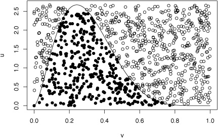
For instance, the generic accept-reject algorithm is based on a marginalisation argument, namely that the marginal distribution (in X) of the Uniform distribution on the sub-graph of $f$: $$\mathfrak S_f=\{(x,u);\ 0\le u\le f(x)\}$$ is the distribution with density proportional to $f$. This means that to produce an $X\sim f(x)$ one generates both $U$ and $X$, even though $U$ is not used as such and obviously does not appear in the (marginal) distribution of $X$. The accept-reject algorithm generates $(X,U)$ in a larger subgraph like the box in the image above and only keeps the $(X,U)$'s that fall under the curve $f$, i.e. in $\mathfrak S_f$.

In the current case, generating from a joint density $f(x|p)f(p)$ to produce simulations from$$m(x) = \int f(x|p)f(p)\,\text{d}p$$is another type of standard approach to the simulation of complex distributions and follows from the argument that if $(X,P)\sim f(x|p)f(p)$ then $X\sim m(x)$. This is the very definition of the marginal distribution but can also be seen by the "law of the unconscious statistician": $$\mathbb E[h(X)]=\int_{\mathcal X} h(x) m(x)\,\text{d}x = \int_{\mathcal X \times \mathcal P} h(x) f(x|p)f(p)\,\text{d}p\,\text{d}x$$ in that $h(x)$ is a function of $(x,p)$ that is constant in $p$.

If the question is about simulation, rather than Bayesian statistics, since the mcmc tag is (unnecessarily) used, the generation of more variates than needed is quite common in random variate generations and goes under different names, like auxiliary variable models, latent variable models, demarginalisation, &tc.

enter image description here

For instance, the generic accept-reject algorithm is based on a marginalisation argument, namely that the marginal distribution (in X) of the Uniform distribution on the sub-graph of $f$: $$\mathfrak S_f=\{(x,u);\ 0\le u\le f(x)\}$$ is the distribution with density proportional to $f$. This means that to produce an $X\sim f(x)$ one generates both $U$ and $X$, even though $U$ is not used as such and obviously does not appear in the (marginal) distribution of $X$. The accept-reject algorithm generates $(X,U)$ in a larger subgraph like the box in the image above and only keeps the $(X,U)$'s that fall under the curve $f$, i.e. in $\mathfrak S_f$.

In the current case, generating from a joint density $f(x|p)f(p)$ to produce simulations from$$m(x) = \int f(x|p)f(p)\,\text{d}p$$is another type of standard approach to the simulation of complex distributions and follows from the argument that if $(X,P)\sim f(x|p)f(p)$ then $X\sim m(x)$.

If the question is about simulation, rather than Bayesian statistics, since the mcmc tag is (unnecessarily) used, the generation of more variates than needed is quite common in random variate generations and goes under different names, like auxiliary variable models, latent variable models, demarginalisation, &tc.

enter image description here

For instance, the generic accept-reject algorithm is based on a marginalisation argument, namely that the marginal distribution (in X) of the Uniform distribution on the sub-graph of $f$: $$\mathfrak S_f=\{(x,u);\ 0\le u\le f(x)\}$$ is the distribution with density proportional to $f$. This means that to produce an $X\sim f(x)$ one generates both $U$ and $X$, even though $U$ is not used as such and obviously does not appear in the (marginal) distribution of $X$. The accept-reject algorithm generates $(X,U)$ in a larger subgraph like the box in the image above and only keeps the $(X,U)$'s that fall under the curve $f$, i.e. in $\mathfrak S_f$.

In the current case, generating from a joint density $f(x|p)f(p)$ to produce simulations from$$m(x) = \int f(x|p)f(p)\,\text{d}p$$is another type of standard approach to the simulation of complex distributions and follows from the argument that if $(X,P)\sim f(x|p)f(p)$ then $X\sim m(x)$. This is the very definition of the marginal distribution but can also be seen by the "law of the unconscious statistician": $$\mathbb E[h(X)]=\int_{\mathcal X} h(x) m(x)\,\text{d}x = \int_{\mathcal X \times \mathcal P} h(x) f(x|p)f(p)\,\text{d}p\,\text{d}x$$ in that $h(x)$ is a function of $(x,p)$ that is constant in $p$.

Source Link
Xi'an
  • 107.7k
  • 13
  • 190
  • 676

If the question is about simulation, rather than Bayesian statistics, since the mcmc tag is (unnecessarily) used, the generation of more variates than needed is quite common in random variate generations and goes under different names, like auxiliary variable models, latent variable models, demarginalisation, &tc.

enter image description here

For instance, the generic accept-reject algorithm is based on a marginalisation argument, namely that the marginal distribution (in X) of the Uniform distribution on the sub-graph of $f$: $$\mathfrak S_f=\{(x,u);\ 0\le u\le f(x)\}$$ is the distribution with density proportional to $f$. This means that to produce an $X\sim f(x)$ one generates both $U$ and $X$, even though $U$ is not used as such and obviously does not appear in the (marginal) distribution of $X$. The accept-reject algorithm generates $(X,U)$ in a larger subgraph like the box in the image above and only keeps the $(X,U)$'s that fall under the curve $f$, i.e. in $\mathfrak S_f$.

In the current case, generating from a joint density $f(x|p)f(p)$ to produce simulations from$$m(x) = \int f(x|p)f(p)\,\text{d}p$$is another type of standard approach to the simulation of complex distributions and follows from the argument that if $(X,P)\sim f(x|p)f(p)$ then $X\sim m(x)$.