added 154 characters in body
Source Link
kjetil b halvorsen
  • 82.8k
  • 32
  • 201
  • 663
  • The way you specify the spline-smooth function is not correct (imm is what you want to estimate in your optimization effort, I do not see how you could use lm())
  • I could not understand which state you observe: this is important because it drives the likelihood (of course)
  • It might be necessary to impose some constraints to the parameters of the SIR model (for example is imm always positive?  ...I I think so)
rm(list = ls()); graphics.off(); cat("\410")

## Libraries and seed
library(deSolve)
library(splines)
set.seed(1234)

## ODE system
SIR = function(t, state, P)
{
  s = state["s"]
  i = state["i"]
  r = state["r"]
  b  = plogis(predict(B, t) %*% P[-1]) 
  g  = plogis(P[1])
  
  ds = - b * (i) * s
  di = b * (i) * s - g * i
  dr = g * i
  return(list(c(ds, di, dr)))
}

## The set ups & data
Nn = 1e3
t0 = 0
t1 = 40
n  = t1 + 1
tt = seq(t0, t1, len = n)
B  = bs(tt, knots = seq(t0, t1, len = 3), Boundary.knots = c(t0, t1+1)) # boundaryknots: ode goes beyond t0, t1

state = c(s = (Nn - 1)/Nn,
          i = 1/Nn,
          r = 0/Nn)

ap   = (seq(10, -12, len = ncol(B))) 
Psim = c(0.25, ap)
sm   = ode(y = state, times = tt, func = SIR, parms = Psim)
is   = sm[, "i"] 
di   = rpois(n , is * Nn)

## The log-likelihood
llik = function(free){

  parms.ode = free
  ode.model = ode(y = state, times = tt, func = SIR, parms = parms.ode) 
  
  fit  = ode.model[, "i"]
  llik = -sum(dpois(di, lambda = fit * Nn, log = TRUE)) 

  return(llik)
}

## The optimization
initg   = runif(1)
inita   = sort(runif(ncol(B), -20, 20), decreasing = T) # reasonable to expect decrising over time
free    = c(initg, inita)
par.fit = optim(par = free, fn = llik, control = list(maxit = 5e3))

## The Predicitons and plot
Popt = par.fit$par
pred = ode(y = state, times = tt, func = SIR, parms = Popt)

par(mfrow = c(2, 1), mar = c(3,3,3,3))
plot(tt, di, main = "Number of infect")
lines(tt, Nn * pred[, "i"], col = "blue")
legend("topright", c("Observed", "Predicted"), col = c(1, 4), lty = c(0, 1), pch = c(1, -1))

plot(tt, plogis(B %*% ap) , type = "l", main = "Time varying beta")
lines(tt, plogis(B %*% Popt[-1]), col = 2, lty = 2)
legend("topright", c("Simulated", "Estimates"), col = c(1, 2), lty = c(1, 2))
graphics.off(); cat("\410")

## Libraries and seed
library(deSolve)
library(splines)
set.seed(1234)

## ODE system
SIR = function(t, state, P)
{
  s = state["s"]
  i = state["i"]
  r = state["r"]
  b  = plogis(predict(B, t) %*% P[-1]) 
  g  = plogis(P[1])
  
  ds = - b * (i) * s
  di = b * (i) * s - g * i
  dr = g * i
  return(list(c(ds, di, dr)))
}

## The set ups & data
Nn = 1e3
t0 = 0
t1 = 40
n  = t1 + 1
tt = seq(t0, t1, len = n)
B  = bs(tt, knots = seq(t0, t1, len = 3), 
        Boundary.knots = c(t0, t1+1)) 
        # boundaryknots: ode goes beyond t0, t1

state = c(s = (Nn - 1)/Nn,
          i = 1/Nn,
          r = 0/Nn)

ap   = (seq(10, -12, len = ncol(B))) 
Psim = c(0.25, ap)
sm   = ode(y = state, times = tt, func = SIR, parms = Psim)
is   = sm[, "i"] 
di   = rpois(n , is * Nn)

## The log-likelihood
llik = function(free){

  parms.ode = free
  ode.model = ode(y = state, times = tt, func = SIR, 
                 parms = parms.ode) 
  
  fit  = ode.model[, "i"]
  llik = -sum(dpois(di, lambda = fit * Nn, log = TRUE)) 

  return(llik)
}

## The optimization
initg   = runif(1)
inita   = sort(runif(ncol(B), -20, 20), decreasing = T) 
        # reasonable to expect decrising over time
free    = c(initg, inita)
par.fit = optim(par = free, fn = llik, 
                control = list(maxit = 5e3))

## The Predicitons and plot
Popt = par.fit$par
pred = ode(y = state, times = tt, func = SIR, parms = Popt)

par(mfrow = c(2, 1), mar = c(3,3,3,3))
plot(tt, di, main = "Number of infect")
lines(tt, Nn * pred[, "i"], col = "blue")
legend("topright", c("Observed", "Predicted"), col = c(1, 4), 
           lty = c(0, 1), pch = c(1, -1))

plot(tt, plogis(B %*% ap) , type = "l", 
         main = "Time varying beta")
lines(tt, plogis(B %*% Popt[-1]), col = 2, lty = 2)
legend("topright", c("Simulated", "Estimates"), 
         col = c(1, 2), lty = c(1, 2))

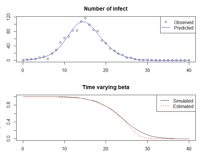
The expected result looks like this (not too bad I think ^_^)   

enter image description here

  • The way you specify the spline-smooth function is not correct (imm is what you want to estimate in your optimization effort, I do not see how you could use lm())
  • I could not understand which state you observe: this is important because it drives the likelihood (of course)
  • It might be necessary to impose some constraints to the parameters of the SIR model (for example is imm always positive?...I think so)
rm(list = ls()); graphics.off(); cat("\410")

## Libraries and seed
library(deSolve)
library(splines)
set.seed(1234)

## ODE system
SIR = function(t, state, P)
{
  s = state["s"]
  i = state["i"]
  r = state["r"]
  b  = plogis(predict(B, t) %*% P[-1]) 
  g  = plogis(P[1])
  
  ds = - b * (i) * s
  di = b * (i) * s - g * i
  dr = g * i
  return(list(c(ds, di, dr)))
}

## The set ups & data
Nn = 1e3
t0 = 0
t1 = 40
n  = t1 + 1
tt = seq(t0, t1, len = n)
B  = bs(tt, knots = seq(t0, t1, len = 3), Boundary.knots = c(t0, t1+1)) # boundaryknots: ode goes beyond t0, t1

state = c(s = (Nn - 1)/Nn,
          i = 1/Nn,
          r = 0/Nn)

ap   = (seq(10, -12, len = ncol(B))) 
Psim = c(0.25, ap)
sm   = ode(y = state, times = tt, func = SIR, parms = Psim)
is   = sm[, "i"] 
di   = rpois(n , is * Nn)

## The log-likelihood
llik = function(free){

  parms.ode = free
  ode.model = ode(y = state, times = tt, func = SIR, parms = parms.ode) 
  
  fit  = ode.model[, "i"]
  llik = -sum(dpois(di, lambda = fit * Nn, log = TRUE)) 

  return(llik)
}

## The optimization
initg   = runif(1)
inita   = sort(runif(ncol(B), -20, 20), decreasing = T) # reasonable to expect decrising over time
free    = c(initg, inita)
par.fit = optim(par = free, fn = llik, control = list(maxit = 5e3))

## The Predicitons and plot
Popt = par.fit$par
pred = ode(y = state, times = tt, func = SIR, parms = Popt)

par(mfrow = c(2, 1), mar = c(3,3,3,3))
plot(tt, di, main = "Number of infect")
lines(tt, Nn * pred[, "i"], col = "blue")
legend("topright", c("Observed", "Predicted"), col = c(1, 4), lty = c(0, 1), pch = c(1, -1))

plot(tt, plogis(B %*% ap) , type = "l", main = "Time varying beta")
lines(tt, plogis(B %*% Popt[-1]), col = 2, lty = 2)
legend("topright", c("Simulated", "Estimates"), col = c(1, 2), lty = c(1, 2))

The expected result looks like this (not too bad I think ^_^)  enter image description here
  • The way you specify the spline-smooth function is not correct (imm is what you want to estimate in your optimization effort, I do not see how you could use lm())
  • I could not understand which state you observe: this is important because it drives the likelihood (of course)
  • It might be necessary to impose some constraints to the parameters of the SIR model (for example is imm always positive?  ... I think so)
graphics.off(); cat("\410")

## Libraries and seed
library(deSolve)
library(splines)
set.seed(1234)

## ODE system
SIR = function(t, state, P)
{
  s = state["s"]
  i = state["i"]
  r = state["r"]
  b  = plogis(predict(B, t) %*% P[-1]) 
  g  = plogis(P[1])
  
  ds = - b * (i) * s
  di = b * (i) * s - g * i
  dr = g * i
  return(list(c(ds, di, dr)))
}

## The set ups & data
Nn = 1e3
t0 = 0
t1 = 40
n  = t1 + 1
tt = seq(t0, t1, len = n)
B  = bs(tt, knots = seq(t0, t1, len = 3), 
        Boundary.knots = c(t0, t1+1)) 
        # boundaryknots: ode goes beyond t0, t1

state = c(s = (Nn - 1)/Nn,
          i = 1/Nn,
          r = 0/Nn)

ap   = (seq(10, -12, len = ncol(B))) 
Psim = c(0.25, ap)
sm   = ode(y = state, times = tt, func = SIR, parms = Psim)
is   = sm[, "i"] 
di   = rpois(n , is * Nn)

## The log-likelihood
llik = function(free){

  parms.ode = free
  ode.model = ode(y = state, times = tt, func = SIR, 
                 parms = parms.ode) 
  
  fit  = ode.model[, "i"]
  llik = -sum(dpois(di, lambda = fit * Nn, log = TRUE)) 

  return(llik)
}

## The optimization
initg   = runif(1)
inita   = sort(runif(ncol(B), -20, 20), decreasing = T) 
        # reasonable to expect decrising over time
free    = c(initg, inita)
par.fit = optim(par = free, fn = llik, 
                control = list(maxit = 5e3))

## The Predicitons and plot
Popt = par.fit$par
pred = ode(y = state, times = tt, func = SIR, parms = Popt)

par(mfrow = c(2, 1), mar = c(3,3,3,3))
plot(tt, di, main = "Number of infect")
lines(tt, Nn * pred[, "i"], col = "blue")
legend("topright", c("Observed", "Predicted"), col = c(1, 4), 
           lty = c(0, 1), pch = c(1, -1))

plot(tt, plogis(B %*% ap) , type = "l", 
         main = "Time varying beta")
lines(tt, plogis(B %*% Popt[-1]), col = 2, lty = 2)
legend("topright", c("Simulated", "Estimates"), 
         col = c(1, 2), lty = c(1, 2))

The expected result looks like this (not too bad I think ^_^) 

enter image description here

added 14 characters in body
Source Link
Gi_F.
  • 1.2k
  • 1
  • 9
  • 14
rm(list = ls()); graphics.off(); cat("\410")

## Libraries and seed
library(deSolve)
library(splines)
set.seed(1234)

## ODE system
SIR = function(t, state, P)
{
  s = state["s"]
  i = state["i"]
  r = state["r"]
  b  = plogis(predict(B, t) %*% P[-1]) 
  g  = plogis(P[1])
  
  ds = - b * (i) * s
  di = b * (i) * s - g * i
  dr = g * i
  return(list(c(ds, di, dr)))
}

## The set ups & data
Nn = 1e3
t0 = 0
t1 = 40
n  = t1 + 1
tt = seq(t0, t1, len = n)
B  = bs(tt, knots = seq(t0, t1, len = 3), Boundary.knots = c(t0, t1+1)) # boundaryknots: ode goes beyond t0, t1

state = c(s = (Nn - 1)/Nn,
          i = 1/Nn,
          r = 0/Nn)

ap   = (seq(10, -12, len = ncol(B))) 
Psim = c(0.25, ap)
sm   = ode(y = state, times = tt, func = SIR, parms = Psim)
is   = sm[, "i"] 
di   = rpois(n , is * Nn)

## The log-likelihood
llik = function(free){

  parms.ode = free
  ode.model = ode(y = state, times = tt, func = SIR, parms = parms.ode) 
  
  fit  = ode.model[, "i"]
  llik = -sum(dpois(di, lambda = fit * Nn, log = TRUE)) 

  return(llik)
}

## The optimization
initg   = runif(1)
inita   = sort(runif(ncol(B), -20, 20), decreasing = T) # reasonable to expect decrising over time
free    = c(initg, inita)
par.fit = optim(par = free, fn =  llik, control = list(maxit = 5e3))

## The Predicitons and plot
Popt = par.fit$par
pred = ode(y = state, times = tt, func = SIR, parms = Popt)

par(mfrow = c(2, 1), mar = c(3,3,3,3))
plot(tt, di, main = "Number of infect")
lines(tt, Nn * pred[, "i"], col = "blue")
legend("topright", c("Observed", "Predicted"), col = c(1, 4), lty = c(0, 1), pch = c(1, -1))

plot(tt, plogis(B %*% ap) , type = "l", main = "Time varying beta")
lines(tt, plogis(B %*% Popt[-1]), col = 2, lty = 2)
legend("topright", c("Simulated", "Estimates"), col = c(1, 2), lty = c(1, 2))
rm(list = ls()); graphics.off(); cat("\410")

## Libraries and seed
library(deSolve)
library(splines)
set.seed(1234)

## ODE system
SIR = function(t, state, P)
{
  s = state["s"]
  i = state["i"]
  r = state["r"]
  b  = plogis(predict(B, t) %*% P[-1]) 
  g  = plogis(P[1])
  
  ds = - b * (i) * s
  di = b * (i) * s - g * i
  dr = g * i
  return(list(c(ds, di, dr)))
}

## The set ups & data
Nn = 1e3
t0 = 0
t1 = 40
n  = t1 + 1
tt = seq(t0, t1, len = n)
B  = bs(tt, knots = seq(t0, t1, len = 3), Boundary.knots = c(t0, t1+1)) # boundaryknots: ode goes beyond t0, t1

state = c(s = (Nn - 1)/Nn,
          i = 1/Nn,
          r = 0/Nn)

ap   = (seq(10, -12, len = ncol(B))) 
Psim = c(0.25, ap)
sm   = ode(y = state, times = tt, func = SIR, parms = Psim)
is   = sm[, "i"] 
di   = rpois(n , is * Nn)

## The log-likelihood
llik = function(free){

  parms.ode = free
  ode.model = ode(y = state, times = tt, func = SIR, parms = parms.ode) 
  
  fit  = ode.model[, "i"]
  llik = -sum(dpois(di, lambda = fit * Nn, log = TRUE)) 

  return(llik)
}

## The optimization
initg   = runif(1)
inita   = sort(runif(ncol(B), -20, 20), decreasing = T) # reasonable to expect decrising over time
free    = c(initg, inita)
par.fit = optim(par = free, fn =  llik)

## The Predicitons and plot
Popt = par.fit$par
pred = ode(y = state, times = tt, func = SIR, parms = Popt)

par(mfrow = c(2, 1), mar = c(3,3,3,3))
plot(tt, di, main = "Number of infect")
lines(tt, Nn * pred[, "i"], col = "blue")
legend("topright", c("Observed", "Predicted"), col = c(1, 4), lty = c(0, 1), pch = c(1, -1))

plot(tt, plogis(B %*% ap) , type = "l", main = "Time varying beta")
lines(tt, plogis(B %*% Popt[-1]), col = 2, lty = 2)
legend("topright", c("Simulated", "Estimates"), col = c(1, 2), lty = c(1, 2))
rm(list = ls()); graphics.off(); cat("\410")

## Libraries and seed
library(deSolve)
library(splines)
set.seed(1234)

## ODE system
SIR = function(t, state, P)
{
  s = state["s"]
  i = state["i"]
  r = state["r"]
  b  = plogis(predict(B, t) %*% P[-1]) 
  g  = plogis(P[1])
  
  ds = - b * (i) * s
  di = b * (i) * s - g * i
  dr = g * i
  return(list(c(ds, di, dr)))
}

## The set ups & data
Nn = 1e3
t0 = 0
t1 = 40
n  = t1 + 1
tt = seq(t0, t1, len = n)
B  = bs(tt, knots = seq(t0, t1, len = 3), Boundary.knots = c(t0, t1+1)) # boundaryknots: ode goes beyond t0, t1

state = c(s = (Nn - 1)/Nn,
          i = 1/Nn,
          r = 0/Nn)

ap   = (seq(10, -12, len = ncol(B))) 
Psim = c(0.25, ap)
sm   = ode(y = state, times = tt, func = SIR, parms = Psim)
is   = sm[, "i"] 
di   = rpois(n , is * Nn)

## The log-likelihood
llik = function(free){

  parms.ode = free
  ode.model = ode(y = state, times = tt, func = SIR, parms = parms.ode) 
  
  fit  = ode.model[, "i"]
  llik = -sum(dpois(di, lambda = fit * Nn, log = TRUE)) 

  return(llik)
}

## The optimization
initg   = runif(1)
inita   = sort(runif(ncol(B), -20, 20), decreasing = T) # reasonable to expect decrising over time
free    = c(initg, inita)
par.fit = optim(par = free, fn = llik, control = list(maxit = 5e3))

## The Predicitons and plot
Popt = par.fit$par
pred = ode(y = state, times = tt, func = SIR, parms = Popt)

par(mfrow = c(2, 1), mar = c(3,3,3,3))
plot(tt, di, main = "Number of infect")
lines(tt, Nn * pred[, "i"], col = "blue")
legend("topright", c("Observed", "Predicted"), col = c(1, 4), lty = c(0, 1), pch = c(1, -1))

plot(tt, plogis(B %*% ap) , type = "l", main = "Time varying beta")
lines(tt, plogis(B %*% Popt[-1]), col = 2, lty = 2)
legend("topright", c("Simulated", "Estimates"), col = c(1, 2), lty = c(1, 2))
deleted 34 characters in body
Source Link
Gi_F.
  • 1.2k
  • 1
  • 9
  • 14
rm(list = ls()); graphics.off(); cat("\410")

## Libraries and seed
library(deSolve)
library(splines)
set.seed(1234)

## ODE system
SIR = function(t, state, P)
{
  s = state["s"]
  i = state["i"]
  r = state["r"]
  b  = plogis(predict(B, t) %*% P[-1]) 
  g  = plogis(P[1])
  
  ds = - b * (i) * s
  di = b * (i) * s - g * i
  dr = g * i
  return(list(c(ds, di, dr)))
}

## The set ups & data
Nn = 1e3
t0 = 0
t1 = 40
n  = t1 + 1
tt = seq(t0, t1, len = n)
B  = bs(tt, knots = seq(t0, t1, len = 3), Boundary.knots = c(t0, t1+1)) # boundaryknots: ode goes beyond t0, t1

state = c(s = (Nn - 1)/Nn,
          i = 1/Nn,
          r = 0/Nn)

ap   = (seq(10, -12, len = ncol(B))) 
Psim = c(0.25, ap)
sm   = ode(y = state, times = tt, func = SIR, parms = Psim)
is   = sm[, "i"] 
di   = rpois(n , is * Nn)

## The log-likelihood
llik = function(free){
  
  parms.ode    = free
  ode.model    = ode(y = state, times = tt, func = SIR, parms = parms.ode) 
  
  # Log-likelihood
  fit  = ode.model[, "i"]
  llik = -sum(dpois(di, lambda = fit * Nn, log = TRUE)) 

    return(llik)
}

## The optimization
initg   = runif(1)
inita   = sort(runif(ncol(B), -20, 20), decreasing = T) # reasonable to expect decrising over time
free    = c(initg, inita)
par.fit = optim(par = free, fn =  llik)

## The Predicitons and plot
Popt = par.fit$par
pred = ode(y = state, times = tt, func = SIR, parms = Popt)

par(mfrow = c(2, 1), mar = c(3,3,3,3))
plot(tt, di, main = "Number of infect")
lines(tt, Nn * pred[, "i"], col = "blue")
legend("topright", c("Observed", "Predicted"), col = c(1, 4), lty = c(0, 1), pch = c(1, -1))

plot(tt, plogis(B %*% ap) , type = "l", main = "Time varying beta")
lines(tt, plogis(B %*% Popt[-1]), col = 2, lty = 2)
legend("topright", c("Simulated", "Estimates"), col = c(1, 2), lty = c(1, 2))
rm(list = ls()); graphics.off(); cat("\410")

## Libraries and seed
library(deSolve)
library(splines)
set.seed(1234)

## ODE system
SIR = function(t, state, P)
{
  s = state["s"]
  i = state["i"]
  r = state["r"]
  b  = plogis(predict(B, t) %*% P[-1]) 
  g  = plogis(P[1])
  
  ds = - b * (i) * s
  di = b * (i) * s - g * i
  dr = g * i
  return(list(c(ds, di, dr)))
}

## The set ups & data
Nn = 1e3
t0 = 0
t1 = 40
n  = t1 + 1
tt = seq(t0, t1, len = n)
B  = bs(tt, knots = seq(t0, t1, len = 3), Boundary.knots = c(t0, t1+1)) # boundaryknots: ode goes beyond t0, t1

state = c(s = (Nn - 1)/Nn,
          i = 1/Nn,
          r = 0/Nn)

ap   = (seq(10, -12, len = ncol(B))) 
Psim = c(0.25, ap)
sm   = ode(y = state, times = tt, func = SIR, parms = Psim)
is   = sm[, "i"] 
di   = rpois(n , is * Nn)

## The log-likelihood
llik = function(free){

  parms.ode = free
  ode.model = ode(y = state, times = tt, func = SIR, parms = parms.ode) 
  
  fit  = ode.model[, "i"]
  llik = -sum(dpois(di, lambda = fit * Nn, log = TRUE)) 

  return(llik)
}

## The optimization
initg   = runif(1)
inita   = sort(runif(ncol(B), -20, 20), decreasing = T) # reasonable to expect decrising over time
free    = c(initg, inita)
par.fit = optim(par = free, fn =  llik)

## The Predicitons and plot
Popt = par.fit$par
pred = ode(y = state, times = tt, func = SIR, parms = Popt)

par(mfrow = c(2, 1), mar = c(3,3,3,3))
plot(tt, di, main = "Number of infect")
lines(tt, Nn * pred[, "i"], col = "blue")
legend("topright", c("Observed", "Predicted"), col = c(1, 4), lty = c(0, 1), pch = c(1, -1))

plot(tt, plogis(B %*% ap) , type = "l", main = "Time varying beta")
lines(tt, plogis(B %*% Popt[-1]), col = 2, lty = 2)
legend("topright", c("Simulated", "Estimates"), col = c(1, 2), lty = c(1, 2))
deleted 38 characters in body
Source Link
Gi_F.
  • 1.2k
  • 1
  • 9
  • 14
Loading
Source Link
Gi_F.
  • 1.2k
  • 1
  • 9
  • 14
Loading