Fitting flexible spline using ODEs

Question

I'm fitting a series of ordinary differential equations (describing movement through disease states: susceptible, infected, recovered) to weekly counts of a disease through time. I'm solving the ODEs using deSolve and fitting using nloptr.

One of the parameters of this model I'd like to estimate is the rate at which individuals move from the recovered state to the susceptible state (imm, in the code below). I want this rate to vary through time.

To do this, I want to fit a flexible/nonparametric spline for this parameter (imm), such that solving the ODEs provides an estimate of the parameters for the spline.

I'm familiar with several R packages for conducting spline regression or for estimating the basis functions for a spline, but can't figure out how to integrate these functions into my ODEs in order to estimate the parameters for the spline using my optimization algorithm. Some of my code is below:

RM = function(t, x, p) {
  imm <- p[1]    

  S <- x[1]    
  I <- x[2]    
  R <- x[3]    

  #total population
  N <- S + I + R
  deaths <- m * N
  births <- deaths
  time <- t

  # define a spline function for the waning immunity parameter
  imm_spl <- lm(imm ~ ns(times, knots = c(seq(0,length(times), by = 180))))

  # Use function to output values at various points along the spline
  imm_spline_values<- predict(imm_spl, times)

  # calculate (predict) the value of the spline at a certain time point
  imm <- imm_spline_values[time]

  # Differential equations
  dS <- births - (beta + m)*S + (imm * R) 
  dI <- (beta * S) - (rec + m) * I
  dR <- (rec * I) - (imm + m) * R 

  res <- c(dS, dI, dR)
  list(res)

}

From here, I'm fitting to the time series data using nloptr and maximum likelihood methods.

Any help would be appreciated.

Answer 1

I worked a bit on your question. I could see only the piece of code you shared (no data or extra detail on your problem). I have following "comments" about your code

• The way you specify the spline-smooth function is not correct (imm is what you want to estimate in your optimization effort, I do not see how you could use lm())
• I could not understand which state you observe: this is important because it drives the likelihood (of course)
• It might be necessary to impose some constraints to the parameters of the SIR model (for example is imm always positive? ... I think so)

To reply to your question (without being too long) I worked on a simplified model :

• I will use a SIR model with fixed population (no birth and deaths)
• I will assume an absorbent R state
• I will not have imm time varying but you will see I will let beta to vary over time
• I will model $\beta(t)$ using B-splines (bs function in R)
• Of course the knots location/number matters: I used 3 internal equally spaced knots (see reference below for an alternative approach)
• I will make sure in my estimation routine that $\beta$ and $\gamma$ are in $[0, 1]$ (see also here Maximum Likelihood Estimate of Infection Model Parameters)
  • So $\gamma$ is the prob. for an infected to recover
  • $\beta$ is the prob. that an interaction between a susceptible and an infected/infectious subject leads to a transmission
• I will make the assumption that the number of infectious $I(t)$ is observed and $I(t) \sim Pois$

A more rigorous inferential approach is discussed here (doi: https://doi.org/10.1093/biostatistics/kxw027). Also the use of P-splines (penalized B-splines) could be beneficial for your problem: it would require to select only the smoothing parameter (not the knots) and would ensure smooth estimates of the time-varying parameter.

The code below reproduces my approach. I left some comments to guide you through it. I hope it is clear enough :-). I apologize if I did not work on your exact ODE system (but I believe it is not the point of your question). I hope it will be easy for you to adapt my example to your needs.

graphics.off(); cat("\410")

## Libraries and seed
library(deSolve)
library(splines)
set.seed(1234)

## ODE system
SIR = function(t, state, P)
{
  s = state["s"]
  i = state["i"]
  r = state["r"]
  b  = plogis(predict(B, t) %*% P[-1]) 
  g  = plogis(P[1])
  
  ds = - b * (i) * s
  di = b * (i) * s - g * i
  dr = g * i
  return(list(c(ds, di, dr)))
}

## The set ups & data
Nn = 1e3
t0 = 0
t1 = 40
n  = t1 + 1
tt = seq(t0, t1, len = n)
B  = bs(tt, knots = seq(t0, t1, len = 3), 
        Boundary.knots = c(t0, t1+1)) 
        # boundaryknots: ode goes beyond t0, t1

state = c(s = (Nn - 1)/Nn,
          i = 1/Nn,
          r = 0/Nn)

ap   = (seq(10, -12, len = ncol(B))) 
Psim = c(0.25, ap)
sm   = ode(y = state, times = tt, func = SIR, parms = Psim)
is   = sm[, "i"] 
di   = rpois(n , is * Nn)

## The log-likelihood
llik = function(free){

  parms.ode = free
  ode.model = ode(y = state, times = tt, func = SIR, 
                 parms = parms.ode) 
  
  fit  = ode.model[, "i"]
  llik = -sum(dpois(di, lambda = fit * Nn, log = TRUE)) 

  return(llik)
}

## The optimization
initg   = runif(1)
inita   = sort(runif(ncol(B), -20, 20), decreasing = T) 
        # reasonable to expect decrising over time
free    = c(initg, inita)
par.fit = optim(par = free, fn = llik, 
                control = list(maxit = 5e3))

## The Predicitons and plot
Popt = par.fit$par
pred = ode(y = state, times = tt, func = SIR, parms = Popt)

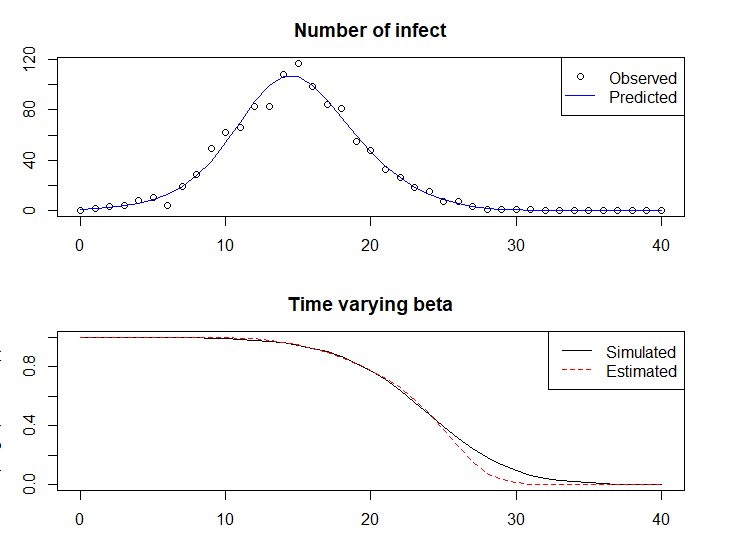
par(mfrow = c(2, 1), mar = c(3,3,3,3))
plot(tt, di, main = "Number of infect")
lines(tt, Nn * pred[, "i"], col = "blue")
legend("topright", c("Observed", "Predicted"), col = c(1, 4), 
           lty = c(0, 1), pch = c(1, -1))

plot(tt, plogis(B %*% ap) , type = "l", 
         main = "Time varying beta")
lines(tt, plogis(B %*% Popt[-1]), col = 2, lty = 2)
legend("topright", c("Simulated", "Estimates"), 
         col = c(1, 2), lty = c(1, 2))

The expected result looks like this (not too bad I think ^_^)