Return to Answer

ns <- 50      # samples of size 50
nt <- 10^4    # compare 10^4 tests

# pU and pT will contain the p-values of the tests
pU <- rep(nt,0)   
pT <- rep(nt,0)

# simulate data and perform tests nt times
for (i in 1:nt) {
  # some funny distribution with three modes
  xy <- c(-1,0,0,0,1)[1+rbinom(ns,4,0.5)]
  y <- rnorm(ns,xy,0.1)
  xz <- c(-1,0,0,0,1)[1+rbinom(ns,4,0.5)]
  z <- rnorm(ns,xz,0.1)

  # perform tests
  pT[i] <- t.test(y,z)$p.value
  pU[i] <- wilcox.test(y,z)$p.value
}

# plot results of different p values
plot(pT,pU, xlim = c(0,0.3), ylim = c(0,0.3),
     xlab = "p value t-test", ylab = "p value Mann-Whitney test", 
     main = "comparing two different tests", pch = 21 , col = 8, bg = 8, cex = 0.5)

# plotting percentage of points in different regions
lines(c(0.05)*c(1,1),c(0,1), col = 2, lty = 2)
lines(c(0,1), c(0.05)*c(1,1), col = 2, lty = 2)
text(0.025,0.025, paste0(sum((pT <= 0.05)*(pU <= 0.05))/nt, " %"), cex = 0.7, col= 2 )
text(0.15,0.025, paste0(sum((pT > 0.05)*(pU <= 0.05))/nt, " %"), cex = 0.7, col= 2 )
text(0.025,0.15, paste0(sum((pT <= 0.05)*(pU > 0.05))/nt, " %"), cex = 0.7, col= 2 )

# plotting the shape of the population distribution
# from which the samples where drawn
t <- seq(-2,2,0.01)
plot(t,0.5^4*dnorm(t,-1,0.1)+0.5^4*dnorm(t,1,0.1)+(1-0.5^3)*dnorm(t,0,0.1), type = 'l',
     xlab = "value", ylab = "density", main = "funny distribution")

ns <- 50      # samples of size 50
nt <- 10^4    # compare 10^4 tests

# pU and pT will contain the p-values of the tests
pU <- rep(nt,0)   
pT <- rep(nt,0)

# simulate data and perform tests nt times
for (i in 1:nt) {
  # some funny distribution with three modes
  xy <- c(-1,0,0,0,1)[1+rbinom(ns,4,0.5)]
  y <- rnorm(ns,xy,0.1)
  xz <- c(-1,0,0,0,1)[1+rbinom(ns,4,0.5)]
  z <- rnorm(ns,xz,0.1)

  # perform tests
  pT[i] <- t.test(y,z)$p.value
  pU[i] <- wilcox.test(y,z)$p.value
}

# plot results of different p values
plot(pT,pU, xlim = c(0,0.3), ylim = c(0,0.3),
     xlab = "p value t-test", ylab = "p value Mann-Whitney test", 
     main = "comparing two different tests", pch = 21 , col = 8, bg = 8, cex = 0.5)

# plotting percentage of points in different regions
lines(c(0.05)*c(1,1),c(0,1), col = 2, lty = 2)
lines(c(0,1), c(0.05)*c(1,1), col = 2, lty = 2)
text(0.025,0.025, paste0(100*sum((pT <= 0.05)*(pU <= 0.05))/nt, " %"), cex = 0.7, col= 2 )
text(0.15,0.025, paste0(100*sum((pT > 0.05)*(pU <= 0.05))/nt, " %"), cex = 0.7, col= 2 )
text(0.025,0.15, paste0(100*sum((pT <= 0.05)*(pU > 0.05))/nt, " %"), cex = 0.7, col= 2 )

# plotting the shape of the population distribution
# from which the samples where drawn
t <- seq(-2,2,0.01)
plot(t,0.5^4*dnorm(t,-1,0.1)+0.5^4*dnorm(t,1,0.1)+(1-0.5^3)*dnorm(t,0,0.1), type = 'l',
     xlab = "value", ylab = "density", main = "funny distribution")

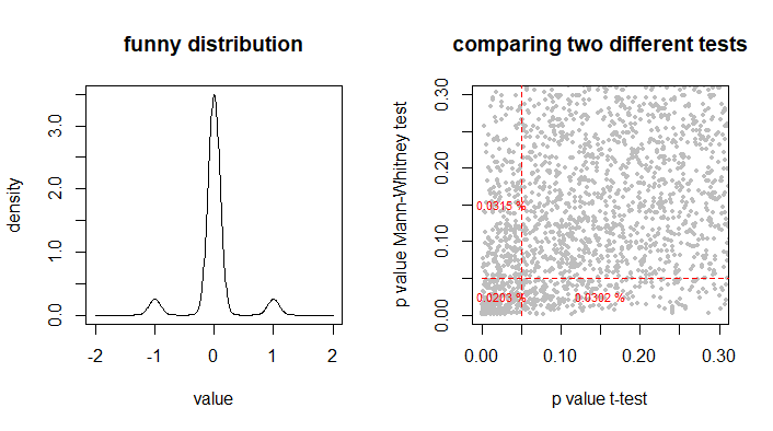
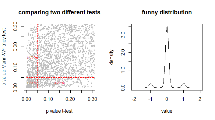
This is demonstrated in the sample below. For some funny shaped population distribution (in order to make the outcome more extreme, with other types of distributions the effect will be less) we take 1000 times two samples of size 50 and compare them based 95% t-test and Mann-Whitney test. Overall, the two tests each reject about 5% of the time the null hypothesis, however they only do this at the same time only in 2% of the cases.

This is demonstrated in the example below. For some funny shaped population distribution (in order to make the outcome more extreme, with other types of distributions the effect will be less) we take 1000 times two samples of size 50 and compare them based 95% t-test and Mann-Whitney test. Overall, the two tests each reject about 5% of the time the null hypothesis, however they only do this at the same time only in 2% of the cases.

The exception is: 1 distribution with infinite variance or very high kurtosis such that they do not approach a normal distribution quickly. 2 when the sample size is small.

In fact: As the sample size gets larger the importance of the normality of the population distribution decreases. But, ironically the probability that a normality test displays a significant difference from a normal distribution increases (because most populations in real life are not exactly normally distributed and given large enough sample size the probability to get a significant difference increases, but 'significance' should not be given any weight, it is about the size of the difference with normality)

The exception is: 1 distribution with infinite variance or very high kurtosis such that the sample mean does not approach a normal distribution quickly. 2 when the sample size is small.