Return to Revisions

About the t-test

With a t-test you are considering whether the means of two samples are significantly different or not.

For sufficiently large samples the value $d = \bar{x_1} - \bar{x_2}$ is approximately Gaussian distributed with some mean $\mu_d$ and $\sigma_d$ and the normalized/standardized value $z= (\bar{x_1} - \bar{x_2})/\sigma$ can be used to test the hypothesis that $\mu_d=0$. (and if the samples are drawn from a normal distribution, then $d$ will be exactly normal distributed)

The value $\sigma_d$ is often unknown and estimated based on the data giving an estimate $\hat\sigma_d$ of the standard deviation of the difference in sample means . So we do not really compute $z=(\bar{x_1} - \bar{x_2})/\sigma$ but instead $t=(\bar{x_1} - \bar{x_2})/\hat\sigma$. The distribution of $t$ does not follow a normal distribution like $z$. If the samples are normally distributed with equal standard deviation then $t$ will be following a t-distribution.

But if the samples are not normally distributed then this will not be the case.

However, if the sample size is large then the distribution will approximate a normal distribution a lot (because the distribution in $\hat\sigma$ is getting more narrow and the distribution in $d$ is getting more like a normal distributed variable). How large the sample needs to be depends on the way how the population distribution deviates from the normal distribution. If the population has large outliers then $d$ will not approach a normal distribution quickly. But if the population is more like a truncated distribution, then the sample will approach a normal distribution quickly.

Example/demonstration

See the below demonstration for the difference in three different population distributions: the normal distribution, a uniform distribution (representing low kurtosis), and a t-distribution (representing high kurtosis). When you have samples of size 50 then there is hardly and difference.

In the image below you see the joint distribution of 1: the estimate of the pooled standard deviation 2: the difference in the means. The t-test draws two boundaries, in this case excluding 5% of the points on the left and right. These boundaries are diagonal. The values $-1.984 \hat\sigma < \bar{x}_1-\bar{x}_2 < 1.984 \hat\sigma$ are considered not significant (with 95% level).

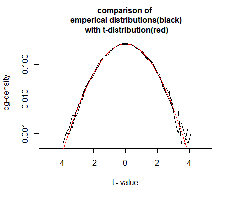
In the above image you see that there is still some reasonable difference in the distribution of $\hat\sigma$, but in the distribution of the values $t=(\bar{x}_1-\bar{x}_2)/\hat\sigma$ there is hardly any difference as you can see below.

So you need not worry much about using a t-test when the samples/population are not exactly normal distributed. The t-test is not very sensitive to deviations like these because with large samples the distribution of the sample mean is gonna approximate a normal distribution no matter what the underlying distribution is. And the distribution of the sample mean scaled by the sample standard deviation is gonna approximate a t-distribution/normal distribution as well because the error in the estimate of the standard deviation is gonna reduce for larger samples.

The exception is: 1 distribution with infinite variance or very high kurtosis such that they do not approach a normal distribution quickly. 2 when the sample size is small.

You can use simulations based on empirical distribution (or maybe you have theoretical consideration that allow you to make assumptions about the population distribution) to verify whether the approximation with a t-distribution make sense.

set.seed(1)

nt <- 10^4  # we do 10^4 trials
ns<- 50     # with samples of size 50

tm <- c()

for (j in 1:3) {
  # generate samples in a matrix
  if (j ==1) {
    x <- matrix(rnorm(nt*ns,0,10),nt)
    y <- matrix(rnorm(nt*ns,0,10),nt)
  }
  if (j == 2) {
    x <- matrix(runif(nt*ns,-sqrt(300),sqrt(300)),nt)
    y <- matrix(runif(nt*ns,-sqrt(300),sqrt(300)),nt)
  }
  if (j == 3) {
    x <- matrix(rt(nt*ns,3),nt)*sqrt(100/3)
    y <- matrix(rt(nt*ns,3),nt)*sqrt(100/3)
  }
  # compute statistics/estimates (means and pooled standard deviation)
  xm <- rowMeans(x)
  ym <- rowMeans(y)
  s_est <- sapply(1:nt, FUN = function(i) sqrt(sd(x[i,])^2 + sd(y[i,])^2)/sqrt(ns))
  
  # perform t-test
  t_est <- sapply(1:nt, FUN = function(i) t.test(x[i,],y[i,])$p.value)
  colours <- hsv(0,(t_est<=0.05),(t_est<=0.05),0.3)
  
  # display in plot
  plot(xm-ym,s_est, ylim = c(0,3), xlim = c(-10,10),
       xlab = "sample mean difference",
       ylab = "sample mean difference \n estimated standard deviation",
       col = colours, bg = colours, pch = 21, cex =0.3)
  sum((t_est<=0.05))/nt
  
  # the limits used by the t-test
  lines(c(0,10),c(0,10)/qt(0.975,ns*2-2))
  lines(-c(0,10),c(0,10)/qt(0.975,ns*2-2))
  tm <- rbind(tm,(xm-ym)/s_est)
  
  title(c("samples from normal distribution",
         "samples from uniform distribution",
         "samples from t-distribution"
         )[j],cex.main = 1)
}

h1 <- hist(tm[1,],breaks = seq(-10,10,0.2))
h2 <- hist(tm[2,],breaks = seq(-10,10,0.2))
h3 <- hist(tm[3,],breaks = seq(-10,10,0.2))
plot(h1$mids,h1$density, type = "l", xlim = c(-5,5), log = "y",
     ylab = "log-density", xlab = "t - value",
     yaxt = "n")
axis(2,at = c(0.001,0.01,0.1,1))
lines(h2$mids,h2$density)
lines(h3$mids,h3$density)
lines(h1$mids,dt(h1$mids,98), col =2)
title("comparison of \n emperical distributions(black)\n with t-distribution(red)", cex.main = 1)