deleted 1 character in body
Source Link
1muflon1
  • 915
  • 5
  • 15

$$Y_t = \phi Y_{t-1}+e_t$$$$Y_t = 0.7 Y_{t-1}+e_t$$

$$Y_t = \phi Y_{t-1}+e_t$$

$$Y_t = 0.7 Y_{t-1}+e_t$$

added 9 characters in body
Source Link
1muflon1
  • 915
  • 5
  • 15

I also tried a following experiment. I estimatedsimulate a random walkfollowing series without time trend:

$$Y_t = Y_{t-1}+e_t$$$$Y_t = \phi Y_{t-1}+e_t$$

I also tried a following experiment. I estimated a random walk without time trend:

$$Y_t = Y_{t-1}+e_t$$

I also tried a following experiment. I simulate a following series without time trend:

$$Y_t = \phi Y_{t-1}+e_t$$

added 2718 characters in body
Source Link
1muflon1
  • 915
  • 5
  • 15

EDIT:

I also tried a following experiment. I estimated a random walk without time trend:

$$Y_t = Y_{t-1}+e_t$$

and compared DF $t$ distribution and rejection region for ADF tests with and without drift term with the results shown on the figure below*.

As the figure below shows the drift distribution of $t$ stat is shifted to the left, but because of the non-standard distribution of DF test under the null each specification has its own critical value.

The critical value for specification (1) should be $t^∗=−1.942$ (green line) and $t^∗=−2.867$ (orange line) - the random walk was simulated with $n=500$. I am just eyeballing it but the rejection regions look to be approximately equally big. That would lead me to conclude that using more general specification does not cause bias (but I don't think this line of reasoning is rigorous)
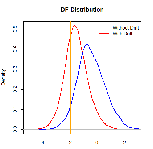
enter image description here

Here is the code used for this simulations:

'%>%'=magrittr::'%>%'
n=1e4
tt_coef = 0.1

ar1 = function(phi, n=500, tt=0, tt_coef=0,sd) {
  y = numeric(500+100)
  for (i in 2:length(y)) {
    y[i] = phi*y[i-1]  + rnorm(1,mean = 0, sd = 1)
  }
  return(tail(y,n)) # first 100 observations burned to remove impact of initial condtns
}

samples_tt = replicate(n,ar1(phi = 0.7,tt = 1, tt_coef = tt_coef, sd = 8),simplify = F)
df_stats_tt = lapply(samples_tt, function(x) urca::ur.df(x,lags = 0,
                                                         type = 'none')@teststat) %>%
  unlist()

samples_rw = replicate(n,ar1(phi = 1, sd = 1),simplify = F)
df_stats_rw = lapply(samples_rw, function(x) urca::ur.df(x,lags = 0,
                                                         type = 'none')@teststat) %>%
  unlist()

df_stats_drift = lapply(samples_rw, function(x) urca::ur.df(x,lags = 0,
                                                            type = 'drift')@teststat[,1]) %>%
  unlist()

sum(df_stats_drift<quantile(df_stats_rw, probs = 0.05))/n
sum(df_stats_tt < quantile(df_stats_rw, probs = 0.05))/n


plot(density(df_stats_drift), type = 'l', lwd = 2, 
     col = 'red', main = 'DF-Distribution', xlab = '')
lines(density(df_stats_rw), type = 'l', lwd = 2, col = 'blue')
abline(v = -1.942, col="orange")
abline(v = -2.867, col="green")
legend('topright', legend = c('Without Drift', 'With Drift'), 
       col = c('blue', 'red'), lwd = 2, bty = 'n')
` 
added 21 characters in body
Source Link
1muflon1
  • 915
  • 5
  • 15
Loading
Source Link
1muflon1
  • 915
  • 5
  • 15
Loading