Do more general specifications of Dickey Fuller lead to bias if true model is more parsimonious?

Question

When I was studying econometrics I was taught that whenever in doubt it is always better to run more general specification both in terms of including drift term or trend term and including lags, as using restrictive specification can lead to bias, whereas having too general specification leads just to loss of power. Regarding lags, I found confirmation of this in Verbeek (2008) A Guide to Modern Econometrics. 2ed pp 277 where he cautions against using ADF test that is too restrictive (in terms of including too little lags).

However, beside appropriately specifying lag terms, DF test has 3 main variants:

No drift, no trend:

$$ \Delta Y_t = (\theta − 1)Y_{t−1} + e_t, \tag{1}$$

Drift, no trend:

$$ \Delta Y_t = \delta + (\theta − 1)Y_{t−1} + e_t, \tag{2}$$

Drift, linear trend:

$$ \Delta Y_t = \delta + (\theta − 1)Y_{t−1} + \beta t + e_t, \tag{3}$$

Of course there could be further variants with quadratic deterministic trend but let us focus only on the ones above.

I was always taught that when in doubt it is best to estimate more general versions of the test (2 or 3), and (1) should only be reserved for the cases where there is absolutely no doubt that model should be parsimonious.

I remember that during my past time series course this was justified by professor referring to the intuition for having more general models in classic regression (in the end DF test is based on regression). In multivariate OLS it is always important to make sure there is no omitted variable bias (OVB), while including too many regressors causes problems as it inflates variances and reduces efficiency, but it is sort of 'lesser evil' relative to OVB. Thus it is generally recommended that when in doubt more general specification should be preferred, and I was taught this extends to the DF test as well.

Is the intuition above correct? If not is it true that using DF with drift when we know that there should be none leads to bias?

PS: I would prefer if it would be possible to also include reference to further literature on this in the answer, if possible, but I am also willing to accept answers that do not do that.

---

EDIT:

I also tried a following experiment. I simulate a following series without time trend:

$$Y_t = 0.7 Y_{t-1}+e_t$$

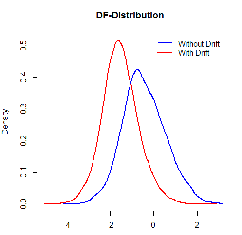
and compared DF $t$ distribution and rejection region for ADF tests with and without drift term with the results shown on the figure below*.

As the figure below shows the drift distribution of $t$ stat is shifted to the left, but because of the non-standard distribution of DF test under the null each specification has its own critical value.

The critical value for specification (1) should be $t^∗=−1.942$ (green line) and $t^∗=−2.867$ (orange line) - the random walk was simulated with $n=500$. I am just eyeballing it but the rejection regions look to be approximately equally big. That would lead me to conclude that using more general specification does not cause bias (but I don't think this line of reasoning is rigorous)

_{Here is the code used for this simulations:}

'%>%'=magrittr::'%>%'
n=1e4
tt_coef = 0.1

ar1 = function(phi, n=500, tt=0, tt_coef=0,sd) {
  y = numeric(500+100)
  for (i in 2:length(y)) {
    y[i] = phi*y[i-1]  + rnorm(1,mean = 0, sd = 1)
  }
  return(tail(y,n)) # first 100 observations burned to remove impact of initial condtns
}

samples_tt = replicate(n,ar1(phi = 0.7,tt = 1, tt_coef = tt_coef, sd = 8),simplify = F)
df_stats_tt = lapply(samples_tt, function(x) urca::ur.df(x,lags = 0,
                                                         type = 'none')@teststat) %>%
  unlist()

samples_rw = replicate(n,ar1(phi = 1, sd = 1),simplify = F)
df_stats_rw = lapply(samples_rw, function(x) urca::ur.df(x,lags = 0,
                                                         type = 'none')@teststat) %>%
  unlist()

df_stats_drift = lapply(samples_rw, function(x) urca::ur.df(x,lags = 0,
                                                            type = 'drift')@teststat[,1]) %>%
  unlist()

sum(df_stats_drift<quantile(df_stats_rw, probs = 0.05))/n
sum(df_stats_tt < quantile(df_stats_rw, probs = 0.05))/n


plot(density(df_stats_drift), type = 'l', lwd = 2, 
     col = 'red', main = 'DF-Distribution', xlab = '')
lines(density(df_stats_rw), type = 'l', lwd = 2, col = 'blue')
abline(v = -1.942, col="orange")
abline(v = -2.867, col="green")
legend('topright', legend = c('Without Drift', 'With Drift'), 
       col = c('blue', 'red'), lwd = 2, bty = 'n')
` 

Answer 1

The problem of model misspecification in the form of too many or too few variables is a bit different in the context of ADF testing than in classical econometric linear regression. In the ADF test, the null distribution of the test statistic varies with model specification (presence/absence of drift and/or trend). If an inappropriate specification is used, the test will have a size distortion and, when size is distorted downward, inferior power. Omitting a variable will lead you to reject the null more often than intended (size distortion) while including too many variables will lead you to fail to reject more often than necessary (inferior power). Depending on how sensitive you are to size distortion vs. power loss, you may find the comparison to OVB more or less appealing.

Side note: what you call linear trend is a trend that is linear in first differences but quadratic in levels.